3.8 Inversion+. Phase consistent tracker.

You are here:

3.8 Inversion+. Phase consistent tracker.

Introduction

This new algorithm is a hybrid method that combines inversion-based flattening with event correlation.

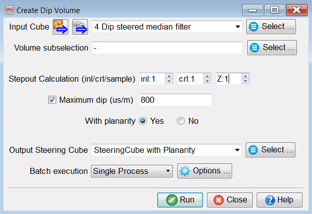
The inversion-based flattening part of the hybrid algorithm is an implementation of the algorithm proposed by Wu and Hale (2015). An initial horizon grid is constructed through one, or more seed positions, after which an inversion algorithm minimizes the error between horizon dips and seismic dips (Fig. 1a). This is done with a conjugate gradient solver. After each iteration loop the horizon grid is re-tied to the input seeds. Seismic dips are pre-computed with a PCA-based algorithm that outputs local dips in the inline and crossline directions. Prior to inversion-based flattening the dip-field is usually smoothed and denoised with a median filter. Optionally, the PCA-based dip computation algorithm outputs a third component called “planarity”. Planarity is a measurement of the local curvedness of the dip field normalized between 0 and 1. High planarity corresponds to good reflections. Low planarity occurs near faults and in noisy sections. Planarity is used by the inversion algorithm to assign higher weights to areas with good reflections.

The similarity-based auto-tracker in this paper starts from one, or more, manually picked seed positions that are snapped to a seismic event. The tracker compares (relative) amplitude differences and cross-correlations between seed traces and traces located at the edges of the growing horizon grid. Positions are added to the grid if the acceptance criteria are met. This tracking mode is used in the exercise in which we compare the three algorithms (next section). In the hybrid algorithm, the decision to add seed positions is based not on relative amplitude differences but only on cross-correlation thresholds.

In the hybrid tracker, the two algorithms are combined. Again the horizon is constrained with one, or more manually picked seeds. In contrast to the inversion-based flattening on dip only, the hybrid algorithm snaps seed positions to the nearest event, i.e. either to a maximum, or to a minimum. An initial horizon grid is constructed through the seed positions and the conjugate gradient solver is started. At various points in the inversion loop, the similarity auto-tracker kicks in to add additional (snapped) seed positions (Fig. 1b). A new horizon grid is constructed through all seeds and the process continues until the end-criteria of the inversion loop are met.

Figure 1 Principle of the hybrid tracker: 1a) An inversion algorithm minimizes the error between horizon grid dips (blue) and pre-computed seismic dips (orange); 1b) The horizon grid is tied to manually picked seed positions (green dots) and auto-generated seeds added by the similarity-based auto-tracker after each inversion cycle (white dots).

Main window for the Inversion + (Phase consistent tracker)

The workflow can be started in three ways:

Insert a new horizon in the table for picking .
Click on the “Pick Seeds” icon and manually pick a set of locations.
Click on the “Load existing Pick Set” icon to open an existing pick set.
Click on the “From Wells” icon and select one or several marker sets and the wells.

Seeds can be added or removed thereafter regardless of the origin of the pickset, either interactively or using the table editor under the Edit options. At least one seed is required for each horizon to be tracked using this tracker.

Inputs

A pre-processed SteeringCube is mandatory. This SteeringCube must be filtered to have less noise. A typical Detailed SteeringCube should be a good starting point.
Seismic cube.
Set of locations (from well makers and/or manually picked positions.
Optional: confidence weight volume (planarity, flipped Thinned Fault Likelihood, …).

Adding Well Markers

Multiple markers from multiple wells can be selected in the Select well markers window . Each selected marker adds a row to the table in the main window. The set of (manually-picked / markers) locations can be QC-ed and edited by pressing the Edit button. To add more picks, select the relevant row, press the Pick Seed button and manually pick positions to add.

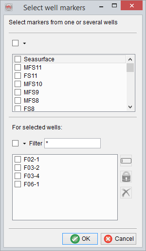
Selection of well markers is done here. Multiple markers can be selected. Each marker will create a horizon.

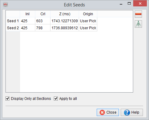
Edit Seeds window will show the origin (user defined or wells) of the picks. By default the seeds are displayed on sections (e.g. inlines/crosslines only). To view in 3D, you may want to toggle this feature off.

Processing Parameters

Manually interpreted faults are provided by setting apply fault dips to yes, which will perform two tasks:
- Calculate fault dips and update the SteeringCube.
- Update the planarity cube at fault location by setting a minimum value of 0.01.
It is not recommended to use the faults without a confidence cube.
A confidence weight volume is optional. It is only required if the interval is faulted. If the given volume has higher weights (e.g. near to 1) at the fault weights, you may flip the weights (1 – input) to minimize the effect of erroneous dips at fault locations.
A planarity volume – as a confidence weight – can be created by pressing the Create button. This will create a SteeringCube with a planarity volume as a third component.

When the batch processing finishes, the right component is chosen to select as a confidence cube.
Correlation method: Event tracking or Dynamic Warping
Correlation window should be small enough to endure a waveform.
Similarity threshold should be 0.6 or higher to track only the high quality events.

A power function is applied to the confidence weights (planarity). Its value is trivial. However, we recommend using a power of 6 or higher. A higher value increases the contrast between faults and continuous reflectors (see below).

The Number of Horizon updates field (max. 100) is the number of times the horizon is changed and horizon dips are re-calculated. The quality of the results increase logarithmically with increasing number of horizon updates. After a certain number of updates, typically 10, the horizon will effectively not change further. If such a situation occurs, we consider that the results are fully converged and the best possible solution is achieved.
The core of the algorithm is a preconditioned Conjugate Gradient ‘CG’ solver, which attempts to solve a system of linear equations. This algorithm is controlled with the following parameters:
- Iterations: The maximum number of iterations the GC solver is run to solve the inverse problem.
- Residual error: The threshold value below which the GC solver stops.
- Preconditioning filter stepout: Is a recursive filter to smooth the horizon and minimizes abrupt jumps (max. 10).
- Inversion Operator Weight: This parameter is trivial and helps in overriding the dips in bad data quality areas. If it is larger than 0 (max. 1), the weighted dip derivatives are subtracted from the dips obtained from horizons to minimize the erroneous dip effects. By default, we do not recommend adding such weights. The Confidence Weight volume mostly controls such effects.

Larger Surveys

For larger datasets (e.g. volume size > 5GB) with limited RAM, we recommend decimation of the results. This can be done in the volume sub-selection. One may upscale the lateral stepouts (Inline/Crossline) to produce a horizon.

Reference

Wu, X., and Hale, D. (2015) Horizon Volume with Interpreted Constraints, Geophysics, v80, Issue 2, IM21-IM33.