3.7 Unconformity Tracker

You are here:

3.7 Unconformity Tracker

This seismic horizon tracker generates one or more horizons from a Steering Cube (dip volume). The tracker uses a constrained, inversion-based algorithm that globally minimizes the error between horizon dips and seismic dips (Wu and Hale, 2015).

A confidence weight volume is recommended for faulted intervals. A good confidence weight volume is given by the “Planarity” attribute. Planarity is computed in the “Faults & Fractures” plugin, It is a measure of “local flatness” of a seismic event. When used as a confidence weight volume in the unconformity tracker it assigns low weights at fault positions and high weights at good reflectors. A flipped discontinuity attribute like similarity, semblance, or Thinned Fault Likelihood can be considered as alternatives to planarity.

The unconformity tracker is a general-purpose horizon tracker that can be used among others to:

Map unconformities (events that change laterally and are therefore difficult to map using conventional amplitude / similarity trackers)..
Map horizons at intra-reservoir scale levels that tie exactly at given well markers.
Fast-track mapping of seismic events, e.g. for constructing a structural framework, to constrain a HorizonCube, or to build low-frequency models for seismic inversion.

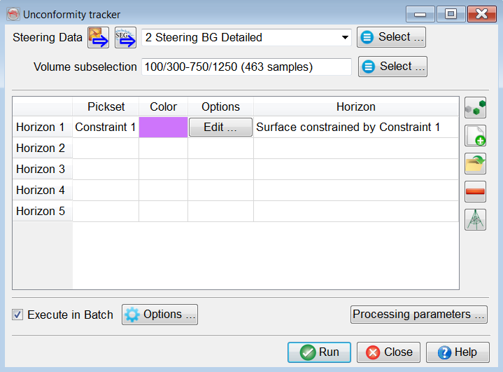
Main window for the Unconformity Tracker

The workflow can be started in three ways:

Insert a new horizon in the table for picking .
Click on the “Pick Seeds” icon and manually pick a set of locations.
Click on the “Load existing Pick Set” icon to open an existing pick set.
Click on the “From Wells” icon and select one or several marker sets and the wells.

Seeds can be added or removed thereafter regardless of the origin of the pickset, either interactively or using the table editor under the Edit options. At least one seed is required for each horizon to be tracked using this tracker.

Inputs

A pre-processed SteeringCube is mandatory. This SteeringCube must be filtered to have less noise. A typical Detailed SteeringCube should be a good starting point.
Set of locations (from well makers and/or manually picked positions.
Optional: confidence weight volume (planarity, flipped Thinned Fault Likelihood, …).

Adding Well Markers

Multiple markers from multiple wells can be selected in the Select well markers window . Each selected marker adds a row to the table in the main window. The set of (manually-picked / markers) locations can be QC-ed and edited by pressing the Edit button. To add more picks, select the relevant row, press the Pick Seed button and manually pick positions to add.

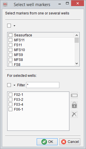
Selection of well markers is done here. Multiple markers can be selected. Each marker will create a horizon.

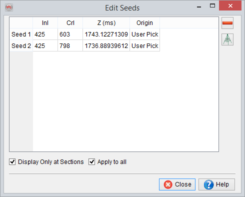
Edit Seeds window will show the origin (user defined or wells) of the picks. By default the seeds are displayed on sections (e.g. inlines/crosslines only). To view in 3D, you may want to toggle this feature off.

Processing Parameters

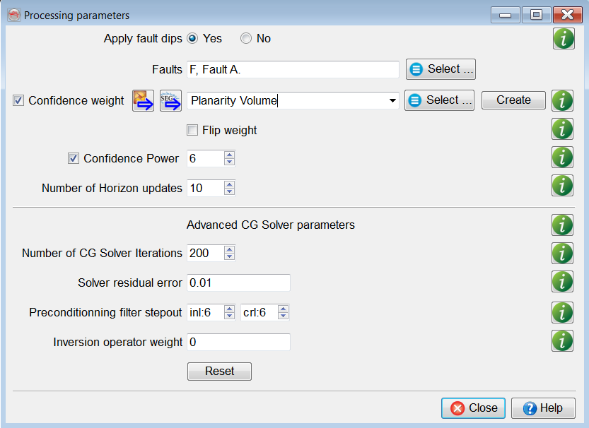
Manually interpreted faults are provided by setting apply fault dips to yes, which will perform two tasks:
- Calculate fault dips and update the SteeringCube.
- Update the planarity cube at fault location by setting a minimum value of 0.01.
It is not recommended to use the faults without a confidence cube.
A confidence weight volume is optional. It is only required if the interval is faulted. If the given volume has higher weights (e.g. near to 1) at the fault weights, you may flip the weights (1 – input) to minimize the effect of erroneous dips at fault locations.
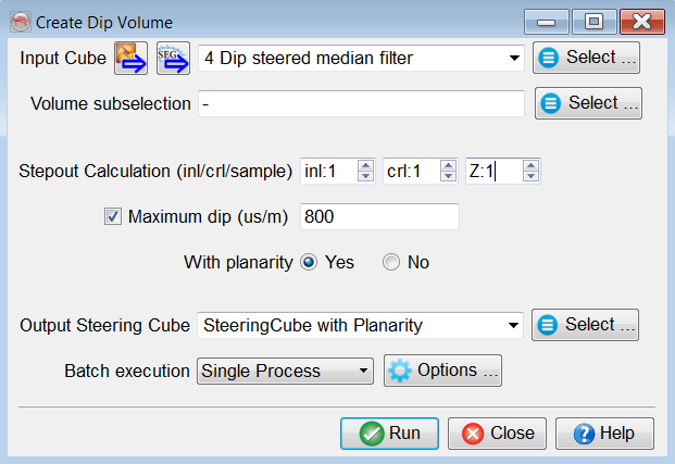
A planarity volume – as a confidence weight – can be created by pressing the Create button. This will create a SteeringCube with a planarity volume as a third component.

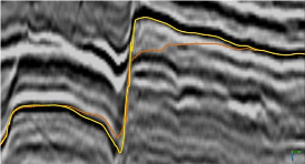
The following result is produced with a confidence weight volume. With a power of 8 (yellow horizon) the event is correctly located when compared with the power of 2 (orange horizon).

When the batch processing finishes, the right component is chosen to select as a confidence cube (see below):

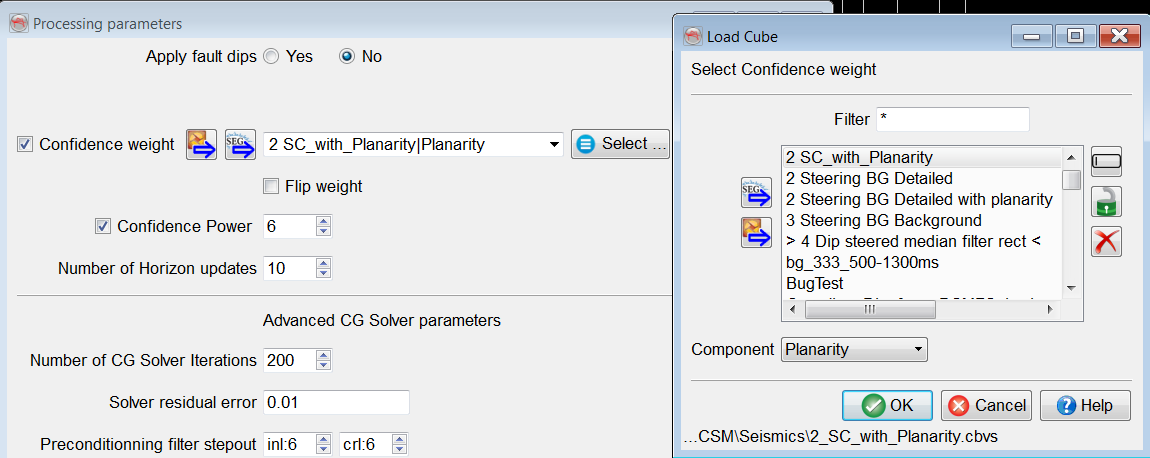
A power function is applied to the confidence weights (planarity). Its value is trivial. However, we recommend using a power of 6 or higher. A higher value increases the contrast between faults and continuous reflectors (see below).

The Number of Horizon updates field (max. 100) is the number of times the horizon is changed and horizon dips are re-calculated. The quality of the results increase logarithmically with increasing number of horizon updates. After a certain number of updates, typically 10, the horizon will effectively not change further. If such a situation occurs, we consider that the results are fully converged and the best possible solution is achieved.
The core of the algorithm is a preconditioned Conjugate Gradient ‘CG’ solver, which attempts to solve a system of linear equations. This algorithm is controlled with the following parameters:
- Iterations: The maximum number of iterations the GC solver is run to solve the inverse problem.
- Residual error: The threshold value below which the GC solver stops.
- Preconditioning filter stepout: Is a recursive filter to smooth the horizon and minimizes abrupt jumps (max. 10).
- Inversion Operator Weight: This parameter is trivial and helps in overriding the dips in bad data quality areas. If it is larger than 0 (max. 1), the weighted dip derivatives are subtracted from the dips obtained from horizons to minimize the erroneous dip effects. By default, we do not recommend adding such weights. The Confidence Weight volume mostly controls such effects.

Larger Surveys

For larger datasets (e.g. volume size > 5GB) with limited RAM, we recommend decimation of the results. This can be done in the volume sub-selection. One may upscale the lateral stepouts (Inline/Crossline) to produce a horizon.

Reference

Wu, X., and Hale, D. (2015) Horizon Volume with Interpreted Constraints, Geophysics, v80, Issue 2, IM21-IM33.