Appendix A - Synthetic Data Generation
Options
- Ray Tracing
- Computation of the Zero Offset Reflection Coefficient
- Computation of the Reflection Coefficient at any non-zero offset
- Elastic Model
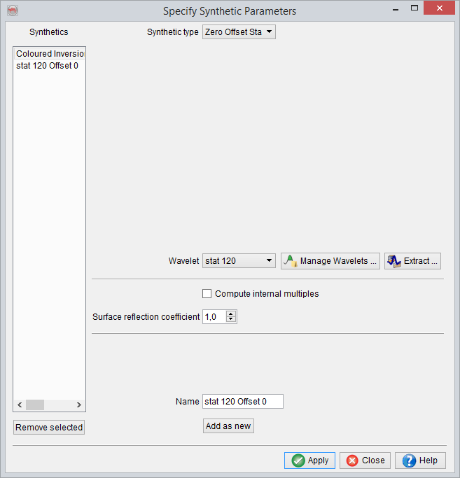
Synthetic seismic data is generated in SynthRock by clicking on the edit icon (![]() ) in the top-left corner of the main Layer Modeling Interface. This will bring up the following window:
) in the top-left corner of the main Layer Modeling Interface. This will bring up the following window:
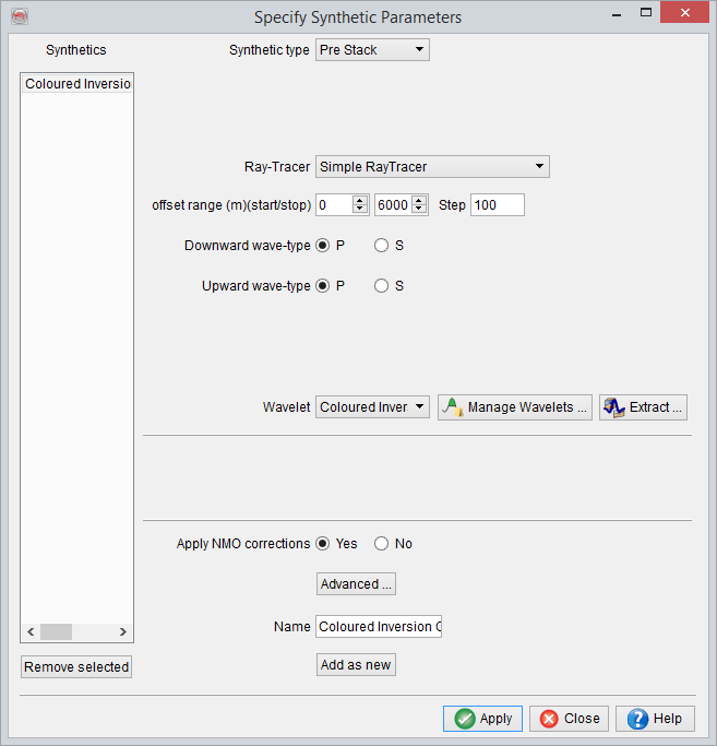
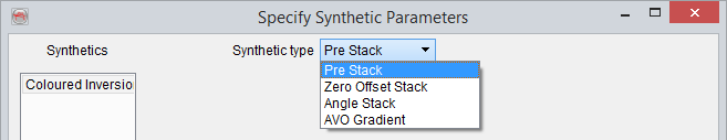
Here various types of synthetic data can be generated: Zero Offset Stack, Pre Stack gathers, Angle Stack and AVO Gradient:
While Zoeppritz equations are used to compute angle-dependent reflectivity; ray tracing is required to compute the angle of incidence, at various interfaces of elastic model, of seismic rays recorded at various offsets. The 2D ray-tracing can be performed in two ways:
Simple Ray Tracer:
The ray is going directly from the source to the depth of the target layer, and up to the receiver in the same way. This does not account for ray bending, or velocity inversions. Here the user has to specify the offset range and the step for creating pre stack gathers; they could in theory be same as defined in acquisition/processing of the seismic data. It can model both Downgoing and Upgoing P-waves and S-waves. Now, ray tracer and Zoeppritz equations have produced angle-dependent or offset-dependent reflectivity traces, which can be convolved with user defined wavelet to produce pre stack gathers. It may be noted that in SynthRock, the conversion from offset domain to angle domain and vice-versa is done using the Vp of the Elastic Model [hyperlink with Elastic Model] (which is essentially the upscaled and time converted Vp log of pseudo-wells).
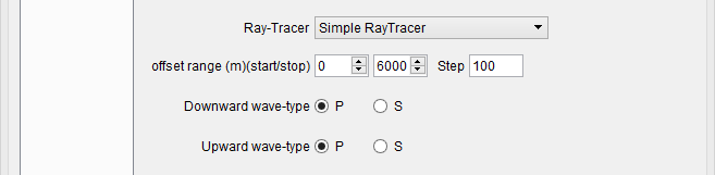
Simple RayTracer parameters
Advanced Ray Tracer (not in the GPL version):
It works in a more sophisticated way than the simple ray tracer. It honours the ray bending according to Snell's law and thus velocity inversions as well. To reduce the processing time, the Elastic Model [hyperlink with Elastic Model] layers may be blocked: Consecutive layers with similar Vp, Vs and Density values are concatenated together, as defined by the threshold. For example the default threshold is 1%, which means if there is less than 1% difference in the elastic model values of two layers, they will be blocked. The ray is propagated in a straight line inside a concatenated layer.
It is also possible to compute internal multiples in the advanced ray tracer. Furthermore, incorporation of spherical divergence, is also possible, by defining the spreading geometry as either "Distance" or "Distance*Vint" .
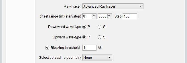
Advanced RayTracer parameters
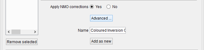
Afterward, NMO corrections can also be applied to create NMO corrected synthetic gathers. Here in the Advanced options, one can specify the % stretch mute typically applicable at far offsets. If the length of a full seismic waveform increases by more than the mute %, it will get muted. Moreover, the taper-length of the muting function, can be defined under this advanced options menu of NMO corrections:
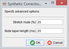
Advanced RayTracer: Advanced corrections options
Computation of the Zero Offset Reflection Coefficient For the simplest Zero Offset Stack, calculation of reflection coefficient at any interface is done using the simple formula:
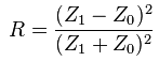
where Z1 and Z0 are the impedance of the top and bottom layers, respectively. These layers are basically upscaled and time converted version of various logs (Rho, Vp and Vs) in pseudo-well models, and as such comprise the Elastic Model [hyperlink with Elastic Model] for synthetic seismic generation. The upscaling is done using the Backus averaging algorithm in depth, but at a (variable) depth sampling rate which is equivalent to the seismic sample rate in time. Depth-to-time conversion of the pseudo-well logs, is done using the velocity model of the pseudo-wells itself.
Backus upscaling is done only for Vp, Vs and Density logs (and other logs based on them e.g. AI, LambdaRho, MuRho etc.). All other logs e.g. Phi, Sw etc. are upscaled using thickness weighted averaging (i.e. weights used for the averaging are the thicknesses of various pseudo-well layers) and are afterwards converted into time (using the velocity model of the pseudo-wells), at survey sample rate. A Nyquist filter, as defined by the survey sample rate is also applied on these time converted rock property traces; e.g. if seismic survey sampling is at 4 ms, Nyquist filter will allow a maximum frequency of 125Hz. These are accessible to user in real-time on the Variable Density View:
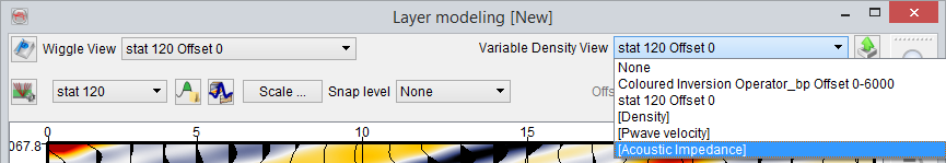
Now, computation of above described reflection coefficient, at all the possible acoustic impedance contrasts in upscaled pseudo-well layers, gives rise to a reflectivity trace in time.
This reflectivity trace is then convolved with a user defined wavelet, to create the Zero Offset Stack for all the pseudo-well models:
Computation of the Reflection Coefficient at any non-zero offset Pre Stack data (i.e. offset gathers) can be generated in OpendTect using full Zoeppritz equations and ray tracing (simple or advanced).
Full Zoeppritz equations are used to compute angle-dependent reflectivity from the elastic model (i.e. upscaled and time converted version of various logs (Rho, Vp and Vs) from pseudo-wells) at various interfaces as:
(above images are from Wikipedia)
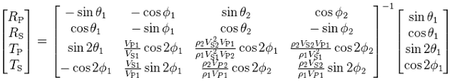
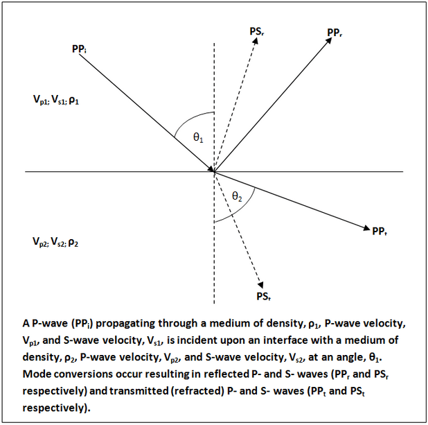
(above images are from Wikipedia)
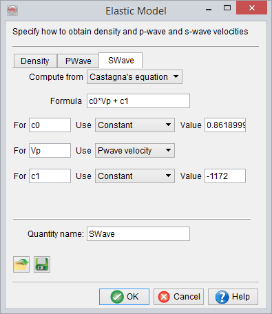
This Elastic Model can be accessed by clicking the ![]() icon, just left of 'Wavelet'. This model isrequired by OpendTect for generating synthetic seismic data (both zero offset stack and pre stack gathers). The elastic model essentially tells the software which quantities to use for the reflection coefficient computation and ray tracing, in terms of Density, Vp and Vs:
icon, just left of 'Wavelet'. This model isrequired by OpendTect for generating synthetic seismic data (both zero offset stack and pre stack gathers). The elastic model essentially tells the software which quantities to use for the reflection coefficient computation and ray tracing, in terms of Density, Vp and Vs:
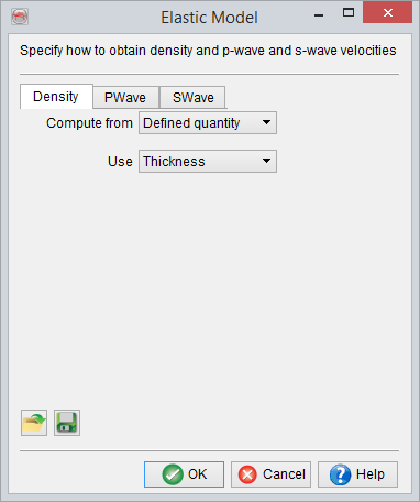
If "Compute from: Defined quantity" is chosen, OpendTect can use appropriate (upscaled and time converted) quantities from pseudo-wells. User can also chose to compute missing quantities (not modeled in pseudo-wells) using pre-filled rock-physics relations, e.g. Vs from Vp using Castagna's equation: