3.4.4 Seismic Image Regression (Supervised 2D and 3D)

A Seismic Image Regression model maps a seismic image (1D, 2D, 3D) to an image with continuous values of similar size. A mapping of seismic inputs (e.g. Acoustic Impedance) to a rock property, such as Porosity, is an example of a Regression model.

These workflows are categorized as supervised methods in that the input data set(s) and the target data are provided to facilitate training. Application of the trained model delivers a new volume (3D seismic) or a new attribute to a line set (2D seismic). We will discuss the workflow and user interface components on the basis of a 3D example.

The objective of this workflow is to interpolate seismic traces where those traces are missing. The model will have to learn how to recreate an image from example images containing blank traces. Therefore, we need an input data set in which we have deliberately blanked some of the traces. In our workflow we do this by randomly blanking approx. 33% of all traces (see caption of the image below for details on how this can be done in OpendTect).

 

In this example workflow we train a 2D Unet but you can equally well train a 3D Unet. The differences between 2D and 3D Unets are as follows:

1. A 2D model trains much faster (hours vs days)

2. 2D models can be trained on workstations with less GPU / CPU capacity

3. Interpolation results are comparable although 2D interpolation may introduce some striping (like a footprint)

4. Application of a trained 3D model is much faster than a trained 2D model (minutes vs hours)

Randomly blanked traces. To train our 2D Unet regression model we create a data set with 33% randomly blanked traces. From this cube we extract examples for training in a restricted area (insert time-slice). The trained model is applied to the entire volume, whereby the area from which no examples are extracted acts as blind test area. The real value is of course when we apply the trained model to an area with real missing traces (which we don’t have in this case). Random blanking (replacing the values with hard zeros) is done in OpendTect’s Attribute engine and can be done in different ways. In this case: 1) Math attribute with formula: “randg(1)”. This generates random values with a Gaussian distribution and 1 standard deviation; 2) Apply this attribute to a horizon and save as horizon data; 3) Horizon attribute that retrieves the random values from the saved horizon data. A Horizon attribute replaces a value at an inline, crossline position with the value extracted from the given horizon; 4) Math attribute with formula: “abs(value)> 1 ? 0: seis”. We assign the retrieved horizon data to the variable “value” and the seismic data to “seis”. This attribute assigns values larger than the absolute value of 1 standard deviation to zero while all other values are given the value of the seismic data.

 

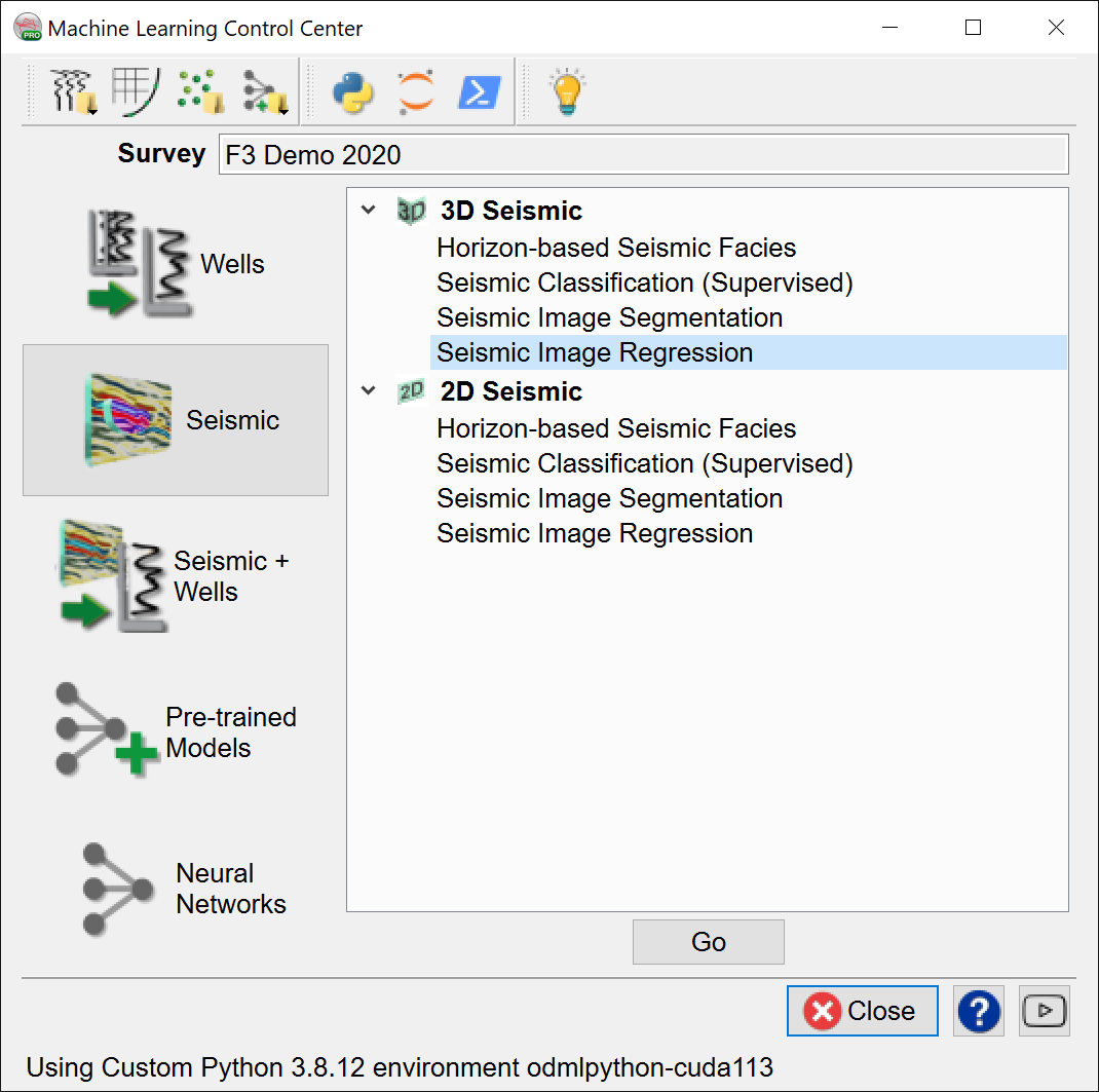
Select the Seismic Image Regression workflow and press Go.

 

Extract Data:

Press the Select button to start the extraction process for the input data.

The “Deep Learning Target Seismic Definition” window pops up. Press the + icon and select the target seismic volume containing the labels. In the example this volume is called “Seismic”.

Note: it is possible to create a Training Set from examples extracted from multiple surveys. To do this, press the + icon again and select the target volume to add to the table below. Repeat until you have selected all data sets to use.

 

The selection can be Saved, retrieved (Open) and modified (Edit) using the corresponding icons. Remove deletes the selection file from the database.

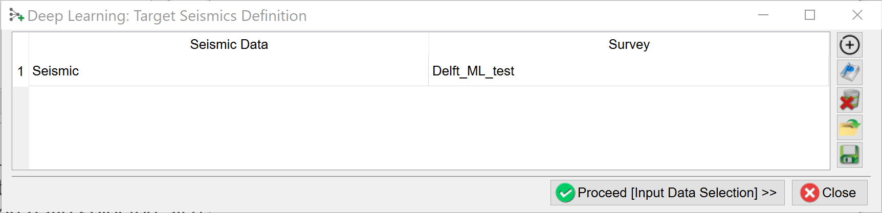
When you are done press Proceed (Input Data Selection). The “Input seismic for prediction” window pops up.

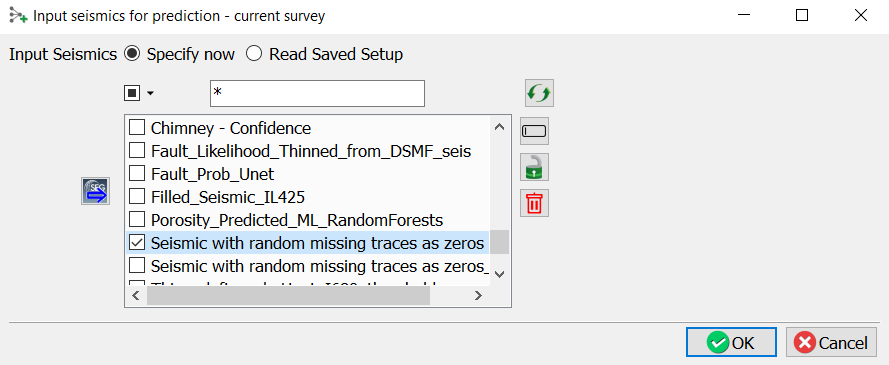
Select the input seismic data and press OK.

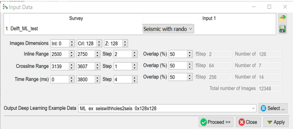
In the “Input Data” window select the dimensions of the input features.

 

Image Dimensions are the number of samples in inline, crossline and Z directions.

Examples:

• Inl: 0; Crl: 128, Z: 128 - extracts 2D images along inlines with dimensions 128 x 128 samples

• Inl: 64, Crl: 64, Z: 64 - extracts cubelets of 6464x64 samples.

The examples (images) are extracted from the specified Inline, Crossline and Time Ranges. Step is the sampling rate in the bin (time) directions. The Overlap determines how much overlap there is between neighboring images. The total number of images is given on the right-hand side of the window. You can control this number by playing with the ranges and overlap parameters.

Specify the name of the Output Deep Learning Example Data and press Proceed to start the extraction process.

When this process is finished you are back in the “Seismic Image Transformation” start window. The Proceed button has turned green. Press it to continue to the Training tab.

 

Training:

When you already have stored data, you can start in the Training tab with Select training data (Input Deep Learning Example data).

Under the Select training data there are three toggles controlling the Training Type:

• New starts from a randomized initial state.

• Resume starts from a saved (partly trained) network. This is used to continue training if the network has not fully converged yet.

• Transfer starts from a trained network that is offered new training data. Weights attached to Convolutional Layers are not updated in transfer training. Only weights attached to the last layer (typically a Dense layer) are updated.

 

After the training data is selected the UI shows which models are available. For seismic image workflows we use Keras (TensorFlow).

Check the Parameters tab to see which models are supported and which parameters can be changed.

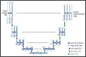
The dGB Unet is an auto-encoder - decoder type of Convolutional Neural Network. The architecture is shown schematically below.

The following training parameters can be set in the Parameters tab:

Batch Size: this is the number of examples that are passed through the network after which the model weights are updated. This value should be set as high as possible to increase the representativeness of the samples on which the gradient is computed, but low enough to have all these samples fit within the memory of the training device (much smaller for the GPU than the CPU). If we run out of memory (raises a python OutOfMemory exception), lower the batch size!

Note that if the model upscales the samples by a factor 1000 for instance on any layer of the model, the memory requirements will be upscaled too. Hence a typical 3D Unet model of size 128-128-128 will consume up to 8GB of (CPU or GPU) RAM.

Epochs: this is the number of update cycles through the entire training set. The number of epochs to use depends on the complexity of the problem. Relatively simple CNN networks may converge in 3 epochs. More complex networks may need 30 epochs, or even hundreds of epochs. Note, that training can be done in steps. Saved networks can be trained further when you toggle Resume.

Patience: this parameter controls early stopping when the model does not change anymore. Increase the patience to avoid early stopping.

Initial Learning rate: this parameter controls how fast the weights are updated. Too low means the network may not train; too high means the network may overshoot and not find the global minimum.

Epoch drop: controls how the learning rate decays over time.

Decimate Input: This parameter is useful when we run into memory problems. If we decimate the input the program will divide the training examples in chunks using random selection. The training is then run over chunks per epoch meaning the model will eventually have seen all samples once within one epoch, but only no more than one chunk of samples will be loaded in RAM while the training is performed.

 

After model selection, return to the Training tab, specify the Output Deep Learning model and press the green Run button. This starts the model training. The Run button is replaced in the UI by Pause and Abort buttons.

The progress can be also followed in a text log file. If this log file does not start automatically, please press the log file icon in the toolbar on the right-hand side of the window.

Below the log file icon there is a Reset button to reload the window. Below this there are three additional icons that control the Bokeh server, which controls the communication with the Python side of the Machine Learning plugin. The server should start automatically. In case of problems it can be controlled manually via the Start and Stop icons. The current status of the Bokeh server can be checked by viewing the Bokeh server log file.

When the processing log file shows “Finished batch processing”, you can move to the Apply tab.

 

 

Apply:

Once the Training is done, the trained model can be applied. Select the trained model and press Proceed.

The Apply window pops up. Here you optionally apply to a Volume subselection.

You can run on GPU or CPU depending on the Predict using GPU toggle. Running the application on a GPU is many times faster than running it on a CPU. Press Run to create the desired outputs. The images below compare the original data with the Unet reconstructed result from input with blanked traced. The line is extracted from the blind test area.