11.16 Mathematics

Name

Mathematics -- Attribute that returns the result of a user-defined mathematical expression

Description

The Mathematics attribute is a way to combine data from stored data and attributes into a new data.

The input data can be volumes, 2D lines or well logs. The output data has always the same dimension (3D, 2D, 1D respectively) as the input, with the exception that 3D and 2D attributes can also be computed along surfaces (horizons and faults). The mathematical expression is calculated at each sample position.

Input Parameters

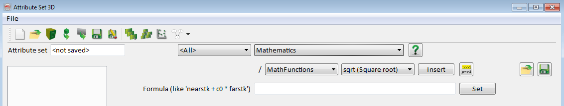
A mathematical expression is specified in the Formula text field with variables, constants, numerical values and/or recursive operators.

• Constants must start with the letter C and be following by a number: C1, C5, C9... The number does not necessarily start at 0 and does not have to be consecutive. Constants can be evaluated just like stepouts and time gates for the other attribute. They are not available for logs creation
• Variables expressions can be any string: seis, energy, sim, ... They can be called with a number between brackets like seis[-1] or seis[4], in which case the value represents a shift in number of samples. seis[-1] represents seis on the sample above, seis[4] represents seis four samples below
• Recursive expressions are a way to call back the result of the mathematical formula on a sample above for computation. This result is called with the expression OUT[-i] (case insensitive) where i is a number of samples

There is no limit in number of variables/constants used in an expression.

There are special constants for which it is not necessary to provide the numerical value: DZ is the sampling rate of the input data, Inl and Crl are respectively the inline and crossline numbers of the current trace. The special constant are case sensitive.

Mathematics attributes containing a recursive equation should only be applied to the full volume/lines, not along a surface because of the integration length.

Parentheses ( ) are allowed. Once the mathematical expression has be entered you must press Set. Then a table will appear where you will be able to assign data to the variables and values to the constants and recursive settings: Start time (or depth) of the recursive function and value at this time.

Supported operators are:

+, -, *, /, ^, >, <, <=, >=, ==, !=, && (and), || (or), |xn |(absolute value), cond ? true stat : false stat.

Supported mathematical functions are:

sin(), cos(), tan(), asin(), acos(), atan(), ln(), log(), exp(), sqrt(), min(), max(), avg(), sum(), med(), var(), rand(v) and randg(std).

Where avg is the average, med is the median, and var is the variance of the input parameters. The input parameters in parentheses should be separated by a comma.

The function rand(v) gives a random number from a uniform distribution between 0 and v. The function randg(std) generates a random number from a Gaussian (normal distribution) with standard deviation std and expectation 0.

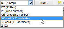
Supported constants are:

pi (3.1415927), undef or null (The OpendTect undefined value: 1e+30), e (2.71...), DZ (Z step), Inl (Inline number), Crl (Crossline number), XCoord (X Coordinate), YCoord (Y Coordinate), Z (Z value), THIS, seis[-1]

In addition it is possible to make logical operations using IF .. THEN .. ELSE statements. The following syntax must be used:

CONDITION ? OUTPUT IF TRUE : OUTPUT IF FALSE

The three parts can be any set of variables and/or constants. IF..THEN..ELSE statements can be embedded like here:

CONDITION1 ? TRUE : (CONDITION2 ? TRUE : FALSE)

Other options

Predefined functions, constants, and operators can be inserted into the 'Formula' field using a combination of the drop-downs, followed by the 'Insert' button. These are grouped so:

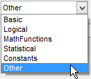
The grouping 'Other' contains the above.

Pressing this button, , will open the 'Rock Physics' library of formulas. Clicking 'Ok' in this additional window will directly insert the chosen formula into the 'Formula' field.

Formulas in Mathematics can be saved () and loaded from a stored location ().

Examples of expressions

• X0 == X1 returns 1 if X0 equals X1, 0 is returned if the statement is false, i.e. X0 is not equal to X1
• X0 != X1 returns 1 if X0 is not equal to X1 and 0 if X0 equals X1
• X0 && X1 returns 1 if X0 and X1 are not equal to 0. If one of these equals zero a 0 is returned
• X0 || X1 returns 1 if X0 or X1 is not equal to 0. If both are zero a 0 is returned
• |X0| returns the absolute value of X0
• X0 > 1 ? X1 : X2 means if X0 is larger than 1 return X1, else return X2
• sin(X0) returns the sine of X0

Let's say you have one input cube, say 'Cube1' and one attribute already defined, Energy40, which is the Energy per sample calculated in a [-20,20] ms window around the current sample. Then, you could define 'Damped amplitude' as;

• Select Mathematics attribute
• Enter formula: seis / energy
• Press Set
• Select 'Cube1' for seis and 'Energy40' for energy
• Provide a name for the attribute, and press Add as new

Additional examples

1. Centred differentiation example: Centred differentiation can be coded using the formula (seis[+1]-seis[-1])/(2*DZ) where DZ is the sampling rate. Please note that for lateral shifts the reference shift attribute must still be used.
2. Recursive filters can be created using the syntax "OUT[-i]". The most general form of recursive equation is the following:
   • y[n] = a0*x[n] + a1*x[n-1] + a2*x[n-2] + ...
   • + b1*y[n-1] + b2*y[n-2] + ...
   • where x[] is the input volume, y[] is the output volume and the a's and b's the coefficients. n is the current sample number.
   • In the mathematics attribute the current sample index "n" does not need to be specified. Therefore the equation above can be entered as:
   • c0*x0 + c1*x0[-1] + c2*x0[-2] + c3*OUT[-1] + c4*OUT[-2] + ...
   • where OUT[-1] stands for y[n-1] and OUT[-2] stands for y[n-2]
   • For each instance of OUT[-i] a starting value and attached time/depth must be provided.
   • Two examples of low pass and high pass recursive filters are provided in the default attribute set "Evaluate attributes":
   • "Single pole low pass recursive filter" and "Single pole high pass recursive filter". Best results are achieved when providing an input of impedance or velocity type.
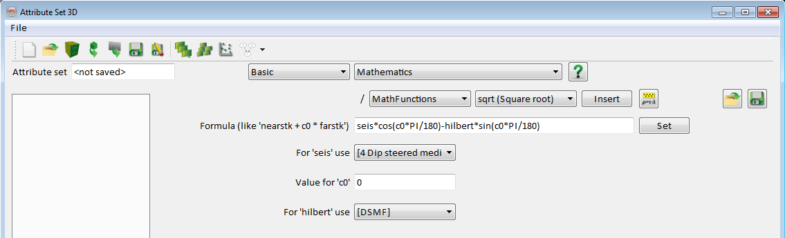
3. The phase rotation is an attribute available in the Evaluate attribute set and in the dGB Evaluate attribute set.
   • This attribute allows the user to apply a phase rotation of any angle to the data.
   • It applies the formula: seis*cos(c0*PI/180)-hilbert*sin(c0*PI/180)
   • where seis is the seismic data
   • hilbert is the Hilbert transform of the seismic data
   • c0 is the applied angle for the rotation
   • c0 is in degrees.