11.23 Scaling

Name

Scaling -- Attribute used for scaling of amplitude

Description

Input Parameters

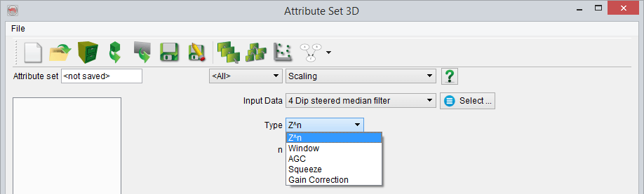
The amplitude of the Input Data can be scaled in five modes:

• Using a time/depth variant weighting function
• Using weight(s) extracted in static time/depth window(s)
• Using Automatic Gain Control (single dynamic window)
• Using Squeeze ('non-clipping' limiter of range input)
• Using Gain Correction (correct/apply gain)

Output

The output amplitudes are always the ratio of the input amplitudes over a weighting function w(i), i being the sample index.

1. Z^n scaling

The weight function is defined by Z^n where Z is the time/depth of the current sample and n is a user-defined exponent:

w(i) = Z(i)^-n where is Z is the time or depth of the ith sample.

The exponent is a float and thus it can be negative, positive and equal to zero (unity operator). An exponent larger than zero will apply a correction proportional to the depth, while an exponent smaller than zero will apply an inversely proportional correction with depth. The output amplitude is the normalized sum of the input amplitude using a weight equal to Z^n.

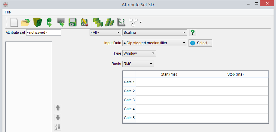
2. Window(s) scaling

The weight function is a step function: w(i) is constant over a static time/depth window, equal to the "basis" value than is computed from the input amplitudes using the following mathematical definitions:

• The Root Mean Square (RMS)
• The arithmetic mean
• The maximum
• A user-defined value (float)
• Detrend. This option removes the trend but rather than doing so following a constant α, it will detrend following αɣ + β. (See: Trend estimation for further info.)

Please note that the window time/depths are float and do not need to be on a sample. The time/depths will be round to the nearest sample when defining the extraction window. Unlike most of the window definitions in the attribute engine you must provide in this scaling attribute absolute time/depths values and not values relative to the actual sample. A weight of 1 (no scaling) will be given to the samples not covered by a user-defined time gate. The weights are cumulative: If several windows overlap the output weight will be the sum of the "basis" output for the samples belonging to multiple windows.

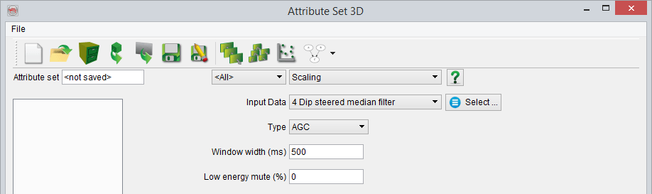
3. Automatic Gain Control scaling

The AGC is a special case of the window scaling. In this case the window is defined relative to the actual sample and the "basis" is the energy value in that sliding window. The window width is a total size, i.e. the relative width corresponds to +/- half of the total window width. The low energy mute will mute the output samples that have an energy lower than a ratio of the trace energy distribution: The energy of the input trace is computed and the output values are sorted per increasing energy value.

Given 1000 samples, the energy of sample 250 (for a low energy mute at 25%) corresponds to the mute level: If the energy computed in the AGC window is lower than this level the value 0 will be output. Otherwise the sum of the squares over the number of (valid) samples will be output. Undefined values are not used for the computation and a zero is output if all values of a time window are undefined. In other words, the energy of all elements within the defined window are calculated and then ranked, then the (user-defined) percentage of the lowest energy levels are muted out.

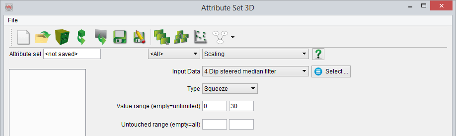
4. Squeeze

The purpose is to put a limit to the value range of the input. Rather than clipping the value (which would be equivalent to a simple Mathematics formula like 'x0 > c0 ? c0 : x0'), the value can be squeezed into a range.

The first parameter is the 'Value range'. it defines the hard limits to the value range. One of these limits may be empty, signifying 'unlimited'.

The second parameter is the 'Untouched range'. If no limits are entered there, Squeeze will degrade to a simple clipping operation. If specified, it will squeeze rather than clip, constraining the squeezing to the ranges outside this range.

For example, Value range [0,10] and untouched range [2,8]. Values outside the [2,8] range will be modified to fit between [0,10]. This means the values in the range [-infinitiy,2] will be squeezed into the range [0,2] via a hyperbolic function. That function is continuous in value (and first derivative) at 2. Similarly, values higher than 8 will go somewhere between 8 and 10.

Example application: predicted porosities. Predictions of porosity tend to have values below 0. To counter this, you could squeeze all values below 1%. Use value range [0, ] and untouched range [1, ]. If you also want a more fuzzy upper limit, starting at 25% to absolute maximum 30, you may specify [0,30] and [1,25].

This is shown in the attribute set below:

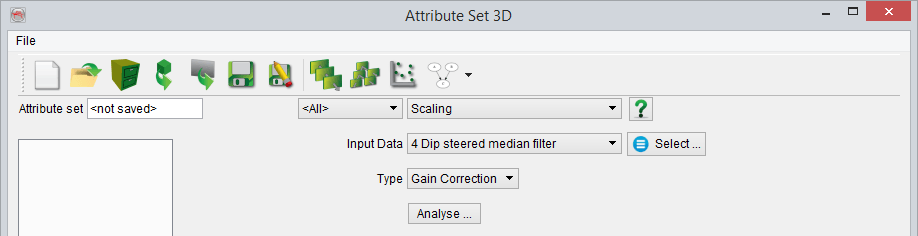
5. Gain Correction

This attribute is used to correct for any undesirable gain applied previously or to apply a new gain function on the seismic data. This is applied by first selecting the input data for gain correction and clicking on Analyse button.

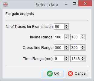
The newly popped Select data window requires specifying a number of random traces in the 'Nr of Traces for Examination' field for visually analyzing and defining the gain behavior in time/depth. The volume from which these random traces will be selected is outlined by modifying the inline, crossline and time ranges. Finally, OK is pressed to begin the examination of the random traces.

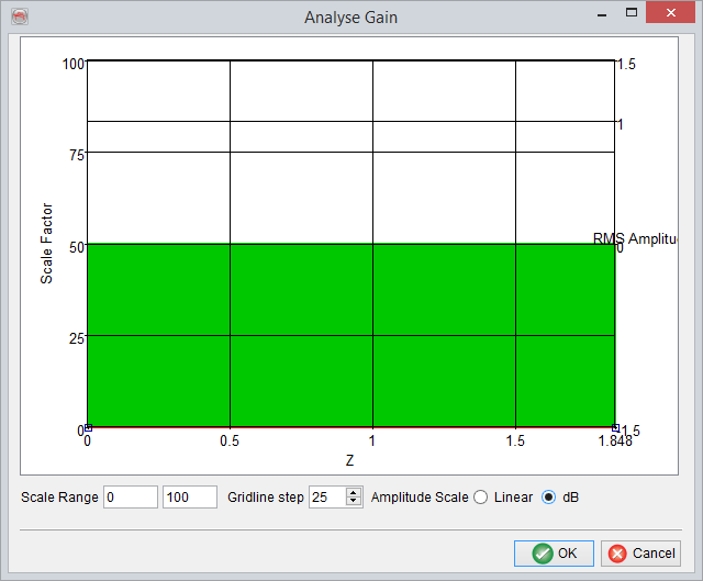
The Analyse Gain window has the 'Z' range (in seconds) of the seismic data as the horizontal axis, while the left vertical axis shows the 'Scale Factor' and the right vertical axis is the 'RMS Amplitude'. The amplitude scale can be set to 'Linear' or 'dB' (i.e. decibel) for visualization purposes. Further, the 'Scale Range' could be changed to use a different scale. The 'Gridline step' could be changed as the name says to modify the gridline steps.

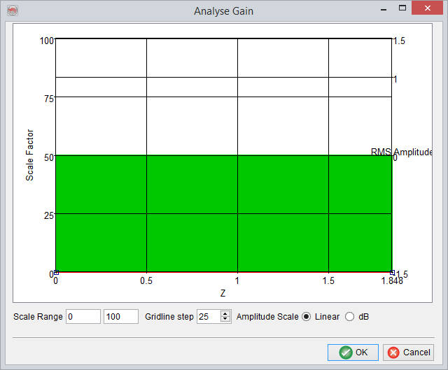
Finally, a 'Gain correction trend' can be defined by moving the red curve such that for any particular 'Z' interval a specific 'Scale Factor' range is used to scale the seismic amplitudes in that interval. For defining boundary points of these intervals user can double click on the red curve and move the curve as desired.

Pressing OK will save the 'Gain correction curve'.