11.26 Spectral Decomposition

Name

Spectral decomposition -- Frequency attribute that returns the amplitude spectrum (FFT) or wavelet coefficients (CWT)

Description

Spectral Decomposition unravels the seismic signal into its constituent frequencies, which allows the user to see phase and amplitude tuned to specific wavelengths. The amplitude component excels at quantifying thickness variability and detecting lateral discontinuities while the phase component detects lateral discontinuities.

It is a useful tool for "below resolution" seismic interpretation, sand thickness estimation, and enhancing channel structures.

Input Parameters

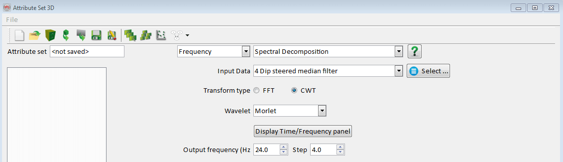
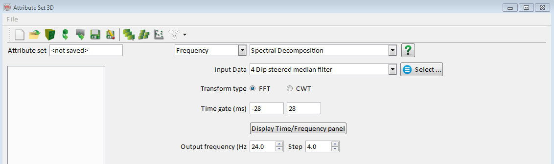
The user can choose between two types of transform:

• FFT the Fast Fourier Transform. The FFT requires a short window (time-gate) and a step-size between the analyzed frequencies. This step can be interpreted as the frequency resolution.
• CWT the Continuous Wavelet Transform. The CWT requires a wavelet type.

When choosing the CWT, you can set the wavelet type:

• Morlet
• Gaussian
• Mexican Hat

In FFT only, the signal within the time-window will be transformed into frequency domain. The given step determines the output resolution, if necessary zeros will be added to acquire this resolution. The amplitude spectrum is calculated for the requested frequency. The time-window slides from top to bottom to cover the complete signal. In an ideal situation, the time-window encompasses one seismic event, which may be a superposition of multiple geological events which interfere in the seismic trace.

Output and Examples

The CWT is defined as the sum over the signal multiplied by a scaled and shifted wavelet. The wavelet is shifted along the signal and at each position the correlation of the wavelet with the signal is calculated. The result is called a wavelet coefficient. The given frequency corresponds to the central wavelet frequency. The step determines the output resolution, which is especially interesting when evaluating this attribute.

Spectral Decomposition (CWT) applied to a horizon. Notice that each index frequency is describing the specific parts of channels (NNE-SSW oriented). Also thinner and thicker parts of horizon along channels are highlighed clearly.

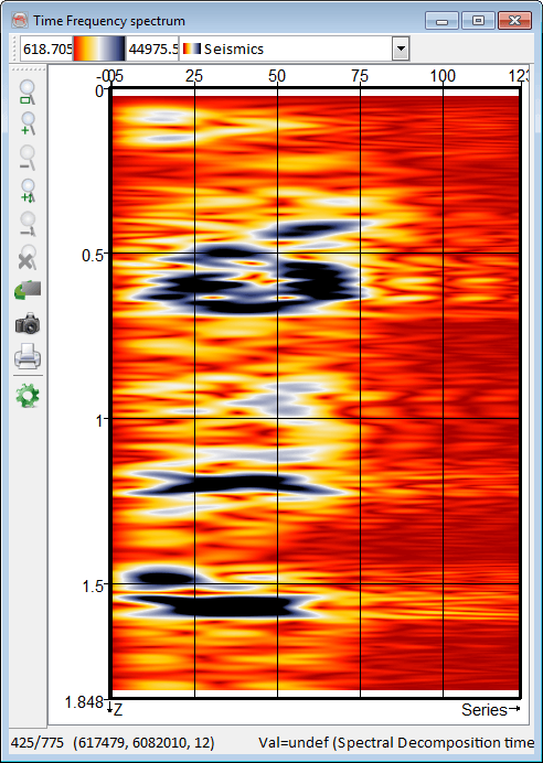
Time-frequency spectrum

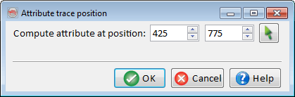
The output frequency is best determined using the time-frequency spectrum panel. This panel displays the spectral decomposition output for all frequencies between 0 and the Nyquist frequency of the data, computed with a step of 1Hz. One must first select a position for this single trace analysis:

The time-frequency is then displayed in a 2D panel like this:

Color blended display:

RGB(A)* blending attribute display is used to create a normalized color-blended display that often show features with greater clarity and enhances a detail map view. Traditionally, it is used to blend the iso-frequency responses (Spectral Decomposition), but a user can blend three/four different attributes that define a spectrum that is comparable. For instance, spectral decomposition outputs the amplitude at discrete frequencies. So, it renders the same output (unit=amplitude). Depending upon a geological condition or the objective, FFT short window or CWT (continuous wavelet transform) can be chosen. Results are best displayed on time/horizon slices, volume.

(* RGB(A)- Red, Green, Blue, (Alpha) -channel)

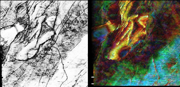
A color blended map view (image on right) of the spectral decomposition (red-10hz, green-20Hz, blue-40hz). Compare the results with the coherency map (image on left). Note that the yellowish colored fault bounder region is thicker as compared to the surrounding regions. The faults throw (red-color) are also clearly observable. Coherency/similarity together with color blended spectral images can reveal better geological information.