11.28 Texture - Directional
Name
Texture - Directional -- a multi-trace attribute that returns textural information based on a statistical texture classification.
Description
Texture- Directional uses the grey level co-occurrence matrix (GLCM) and its derived attributes are tools for image classification that were initially described by Haralick et al. (1973). Principally, the GLCM is a measure of how often different combinations of pixel brightness values occur in an image. It is a method widely used in image classification of satellite images (e.g. Franklin et al., 2001; Tsai et al., 2007), sea-ice images (e.g. Soh and Tsatsoulis, 1999; Maillard et al., 2005), magnetic resonance and computed tomography images (e.g. Kovalev et al., 2001; Zizzari et al., 2011), and many others. Most of these GLCM applications are for classification of 2D images solely. The application of GLCM for seismic data has been a minor topic in comparison to common seismic attributes such as coherence, curvature or spectral decomposition. Today, a high percentage of the available seismic data is 3D seismic. Therefore, it is important for the classification of seismic data to adapt the GLCM calculation to work in the three-dimensional space. Few authors have described the application of GLCM for 3D seismic data with various approaches to this topic (Vinther et al., 1996; Gao, 1999, 2003, 2007, 2008a, 2008b, 2009, 2011; West et al., 2002; Chopra and Alexeev, 2005, 2006a, 2006b; Yenugu et al., 2010; de Matos et al., 2011; Eichkitz et al. 2012, 2013, 2014).
The calculation of GLCM-based attributes can be done in separate space directions. For the 2D case 4 space directions exist. For the 3D case the number of possible space directions is extends to 13. The principal workflow of GLCM-based attribute calculation consists of transformation of the amplitude cube into a grey level cube, the counting of pixel co-occurrences within in a given analysis window, and the calculation of attributes based on the co-occurrence matrix. In Figure 1 the principal calculation of 2D GLCM in four space directions is shown for a sample image.
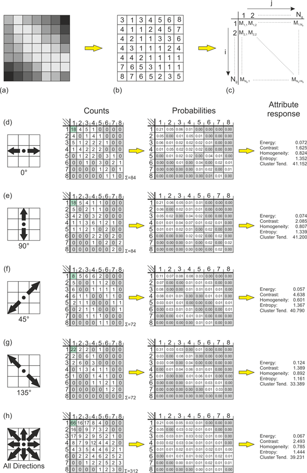
Figure 1: Example for the calculation of grey level co-occurrence matrix-based attributes using eight grey levels for a randomly generated 2D grey-scale image (a). The grey-scales of the image can be represented by discrete values (b). The number of co-occurrences of pixel pairs for a given search window are counted and a grey level co-occurrence matrix (c) is produced. Based on this co-occurrence matrix, several attributes can be calculated. In this example, the grey level co-occurrence matrices are determined for the horizontal (d), the vertical (e), the 45° diagonal (f), the 135° diagonal (g), and for all directions at once (h). The first step in calculation is the determination of co-occurrences (column 2). Zero entries are marked in light grey and the highest value of each matrix is marked in dark grey. It is evident that calculations in single directions lead to sparse matrices. The GLCM is normalized by the sum of the elements to get a kind of probability matrix (column 3). Finally, the probabilities are used for the calculation of GLCM-based attributes. In column 4 the results for Entropy, Contrast, Homogeneity, Entropy, and Cluster Tendency are shown.
In the case of 3D data the number of possible directions increases to 13. In Figure 2 a simple Rubik’s cube is taken to explain the 13 possible directions for a 3D dataset. This Rubik’s cube is build-up of 27 small cubes. The small cube in the center (the turning point in a Rubik’s cube) is the point of interest for which the calculations are performed. This center point is surrounded by 26 neighboring cubes. If we now take the center point and draw lines form it to all neighboring cubes, we get 13 directions on which the neighboring samples are placed.
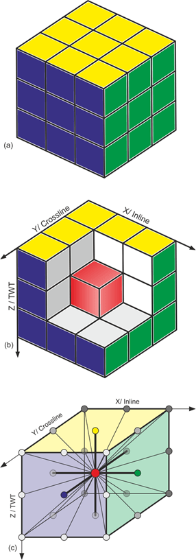
Figure 2: The number of principal neighbors for one sample point can be best explained by looking at a Rubik’s cube (a). The center of the Rubik’s cube (core mechanism for rotating the cube, red box in (b)) has in total 26 neighboring boxes (including diagonal neighbors). These boxes are aligned in 13 possible directions. Analogous to this, a sample point within a seismic sub-volume has 26 neighbors aligned in 13 directions (c). In the developed workflow it is possible to calculate the GLCM along single directions, along combinations of directions (e.g. inline direction, crossline direction, …), or all directions can be calculated at once (after Eichkitz et al., 2013).
Input Parameters
Input Data
The input for the GLCM-based attribute calculation can be any seismic amplitude 3D cube/2D section. In the process of GLCM calculation this amplitude cube is converted to a grey level cube.
Compute Amplitude Range
For the transformation of the amplitude cube to a grey level cube the range of the amplitude values is needed. This can either be inserted manually, or be computed. In the case of computed amplitude range, the amplitude range will be symmetrical around zero.
Number of Grey Levels
The number of grey levels used for the transformation of amplitude cube to grey level cube. Higher numbers generally improve the quality of the GLCM output. Common numbers for the grey levels are 16 to 256.
Number of Traces
The number of traces defines the horizontal analysis window. This horizontal analysis window is always symmetrical around the center trace. Number of traces equal 1 means 1 trace left and right of the center trace (thus 3 traces).
Vertical Search Window
The vertical search window defines the number of samples included in the search window. The vertical size of the analysis window should be according to the average wavelength (Gao, 2007). This is typically in the range of 15 samples (+/- 7 samples).
In total 23 GLCM-based attributes can be calculated (see below in Mathematical description)
Direction of Calculation
The GLCM-based attribute calculation can in principal be done in 13 space directions for 3D input data (4 space directions for 2D data). The algorithm allows the calculation in single directions or the combined calculation of several directions (inline, crossline, time-/depthslice) or all 13 space directions can be calculated at once. Multiple directions give smoother results, but subtle features might be missed. Detailed analysis of single directions might give information about fracturing or facies distribution of the subsurface.
In this process azimuth of 0° is equal to inline direction; azimuth of 90° is equal to crossline direction. Dip of 0° is equal to horizontal direction, dip of 90° is equal to vertical direction.
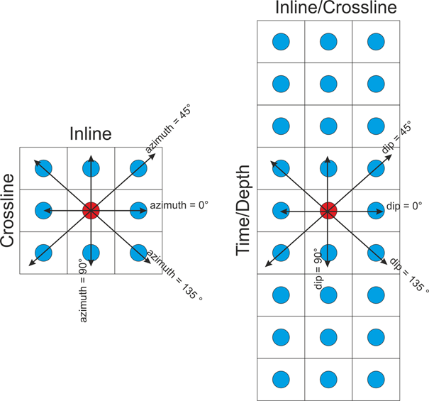
Figure 3: Definition of directions.
GLCM attribute calculation can be done with or without steering. The integration of dip steering generally improves the signal-to-noise ratio in calculated attributes.
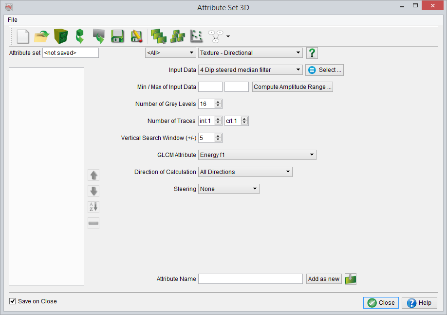
Figure 4: Texture attribute window within OpendTect.
Mathematical description
The GLCM is a measure of how often different combinations of neighboring pixel values occur within an analysis window. For a 2D image the immediate neighboring pixels can be in four different directions (0°, 45°, 90°, and 135°). For the calculation of 2D GLCM the following equation is used:
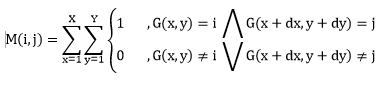
where i and j vary from 1 to Ng (number of grey levels).
In this equation G(x,y) are the center sample points and G(x+dx, y+dy) are the neighboring sample points. Usually, the distance between center and neighboring samples is one, but in general greater distances could also be taken for the calculation. It is, in principal also possible to combine the four principal directions to form an average GLCM. By this approach the spatial variations can be eliminated to a certain degree (Gao 2007). In the case of 3D data the number of possible directions increases to 13. The 3D case implies a modification of the above given equation:
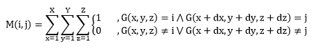
Similar to the 2D case, it is possible to calculate the GLCM in single directions, to combine several directions, or to calculate an average GLCM. Previous works on 3D GLCM calculation use 2D GLCM calculations in various directions and combine the results of these calculations to form a pseudo-3D GLCM attribute cube.
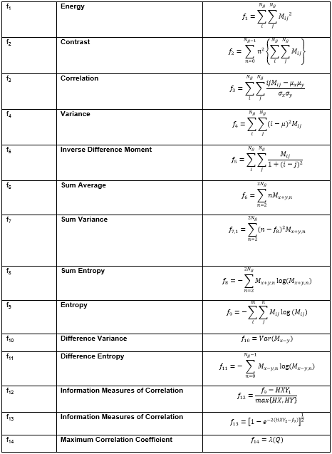
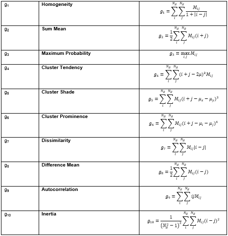
Based on the grey level co-occurrence matrix, it is possible to calculate several attributes. Haralick et al. (1973), in their work, describe 14 attributes that can be calculated from the GLCM. In literature a few more attributes based on the GLCM have been developed (e.g. Soh and Tsatsoulis, 1999; Wang et al., 2010). For the calculation of any of these GLCM-based attributes it is necessary to normalize the GLCM to generate a kind of probability matrix. This is done by dividing each matrix entry by the sum of all entries. The different GLCM-based attributes can be divided into three general groups. The first group is the contrast group and includes measurements such as contrast and homogeneity. All the attributes from this first group are basically a function of the probability of each matrix entry and the difference of the grey levels (i and j). Therefore, these contrast group attributes are related to the distance from the GLCM diagonal. Values on the diagonal (where i and j are the same) result in zero contrast, whereas the contrast increases by increase of distance from the diagonal.
The second attribute group is the orderliness group, which includes attributes such as energy and entropy. Attributes in the orderliness group measure how regular grey level values are distributed within a given search window. In contrast to the first group all attributes from this group are solely a function of the GLCM probability entries.
The third attribute group is the statistics group, which includes attributes such as Haralick et al.’s (1973) measure of mean and variance. These are common mean and variance calculations applied onto the GLCM probabilities.
The following tables summarize all GLCM equations:
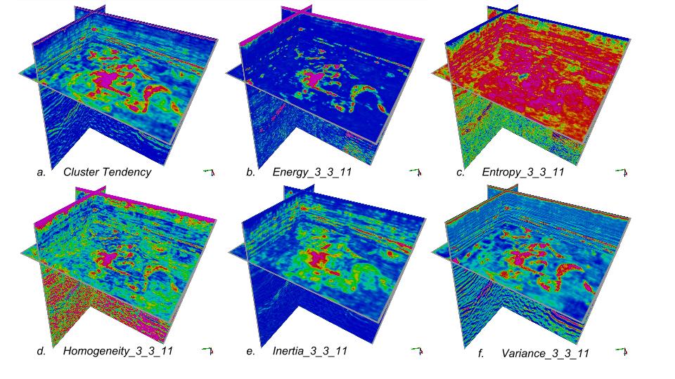
Examples
References
- Chopra, S., and V. Alexeev, 2005, Application of texture attribute analysis to 3D seismic data: 75th SEG meeting, Houston, Texas, USA, Expanded Abstracts, 767-770.
- Chopra, S., and V. Alexeev, 2006a, Application of texture attribute analysis to 3D seismic data: The Leading Edge, 25, no. 8, 934-940.
- Chopra S., and V. Alexeev, 2006b, Texture attribute application to 3D seismic data: 6th International Conference & Exposition on Petroleum Geophysics, Kolkata, India, Expanded Abstracts, 874-879.
- de Matos, M.C., Yenugu, M., Angelo, S.M., and K.J. Marfurt, 2011, Integrated seismic texture segmentation and cluster analysis applied to channel delineation and chert reservoir characterization: Geophysics, 76, no. 5, P11-P21.
- Eichkitz, C.G., Amtmann, J. and M.G. Schreilechner, 2013, Calculation of grey level co-occurrence matrix-based seismic attributes in three dimensions: Computers and Geosciences, 60, 176-183.
- Eichkitz, C.G., de Groot, P. and Brouwer, F., 2014. Visualizing anisotropy in seismic facies using stratigraphically constrained, multi-directional texture attribute analysis. AAPG Hedberg Research Conference “Interpretation Visualization in the Petroleum Industry”, Houston, USA.
- Franklin, S.E., Maudie, A.J., and M.B. Lavigne, 2001, Using spatial co-occurrence texture to increase forest structure and species composition classification accuracy: Photogrammetric Engineering & Remote Sensing, 67, no. 7, 849-855.
- Gao, D., 1999, 3-D VCM seismic textures: A new technology to quantify seismic interpretation: 69th SEG meeting, Houston, Texas, USA, Expanded Abstracts, 1037-1039.
- Gao, D., 2003, Volume texture extraction for 3D seismic visualization and interpretation: Geophysics, 68, no. 4, 1294-1302.
- Gao, D., 2007, Application of three-dimensional seismic texture analysis with special reference to deep-marine facies discrimination and interpretation: Offshore Angola, West Africa: AAPG Bulletin, 91, no. 12, 1665-1683.
- Gao, D., 2008a, Adaptive seismic texture model regression for subsurface characterization: Oil & Gas Review, 6, no. 11, 83-86.
- Gao, D., 2008b, Application of seismic texture model regression to seismic facies characterization and interpretation: The Leading Edge, 27, no. 3, 394-397.
- Gao, D., 2009, 3D seismic volume visualization and interpretation: An integrated workflow with case studies: Geophysics, 74, no. 1, W1-W24.
- Gao, D., 2011, Latest developments in seismic texture analysis for subsurface structure, facies, and reservoir characterization: A review: Geophysics, 76, no. 2, W1-W13.
- Haralick, R.M., Shanmugam, and K. Dinstein, I., 1973, Textural features for image classification: IEEE Transactions on systems, man, and cybernetics, 3, no. 6, 610-621.
- Kovalev, V.A., Kruggel, F., Gertz, H.-J., and D.Y. von Cramon, 2001, Three-dimensional texture analysis of MRI brain datasets: IEEE Transactions on medical imaging, 20, no. 5, 424-433.
- Maillard, P., Clausi, D.A., and H. Deng, 2005, Operational map-guided classification of SAR sea ice imagery: IEEE Transaction on Geoscience and Remote Sensing, 43, no. 12, 2940-2951.
- Soh, L.-K., and C. Tsatsoulis, 1999, Texture analysis of SAR sea ice imagery using gray level co-occurrence matrices: IEEE Transactions on Geoscience and Remote Sensing, 37, no. 2, 780-795.
- Tsai, F., Chang, C.-T., Rau, J.-Y., Lin, T.-H., and G.-R. Liu,, 2007, 3D computation of gray level co-occurrence in hyperspectral image cubes: LNCS 4679, 429-440.
- Vinther, R., Mosegaar, K., Kierkegaard, K., Abatzi, I., Andersen, C., Vejbaek, O.V., If, F., and P.H. Nielsen, 1996, Seismic texture classification: A computer-aided approach to stratigraphic analysis: 65th SEG meeting, Houston, Texas, USA, 153-155.
- Wang, H., Guo, X.-H., Jia, Z.-W., Li, H.-K., Liang, Z.-G., Li, K.-C., and Q. He, 2010, Multilevel binomial logistic prediction model for malignant pulmonary nodules based on texture features of CT image: European Journal of Radiology, 74, 124-129.
- West, B.P., May, S.R., Eastwood, J.E., and C. Rossen, 2002, Interactive seismic facies classification using textural attributes and neural networks: The Leading Edge, 21, no. 10, 1042-1049.
- Yenugu, M., Marfurt, K.J., and S. Matson, 2010, Seismic texture analysis for reservoir prediction and characterization: The Leading Edge, 29, no. 9, 1116-11.
- Zizzari, A., Seiffert, U., Michaelis, B., Gademann, G., and S. Swiderski, 2001, Detection of tumor in digital images of the brain: Proc. of the IASTED international conference Signal Processing, Pattern Recognition & Applications, Rhodes, Greece, 132-137.