3.6 Pre-trained Models
A geophysics library of trained Machine Learning models is released to the users of OpendTect Machine Learning plugin. These pre-trained models can be reused AS IS to solve a wide range of generic problems on unseen data.
Applying such models is easy with no need to train the data, and valuable results can be obtained much faster than through alternative workflows involving reprocessing or expert knowledge.
We will show which type of models are available. As well as examples of seismic and well log models that are applied to blind test data sets.
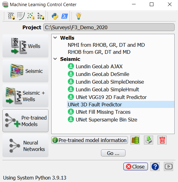
Tools have been developed (in Keras / TensorFlow, PyTorch and Scikit Learn) for importing models into OpendTect’s Machine Learning solution.
 Download status*
 Model information
 Pre-trained model disk locations
 Import models
 Delete models
Researchers & Experimental geoscientists can use these tools to create a proprietary library of trained models that can be shared with operational geoscientists inside their own company.
Because of the size of Machine Learning models, the trained models are stored in our library in the cloud.
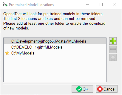
![]() Default download location (can be an on-premise shared network location)
Default download location (can be an on-premise shared network location)
Users have access to meta information such as: model objective, required inputs, generated outputs, model shape, and what examples the model was trained on. Based on this information, users can download models of interest and apply these to their own data. Trained models in the current library originate from dGB and from researchers of Lundin GeoLab (nowadays AkerBP) who granted permission to distribute their seismic models to our users.
Note: All models are 3D Unets trained on synthetic data with shape 128x128x128.
Seismic - UNet 3D Fault Predictor
Predict Fault Likelihood from 3D seismic.
The Unet 3D Fault Predictor, is a powerful and super fast tool to predict faults and fractures in seismic data. This model was trained on synthetic seismic cubelets of 128x128x128 samples.
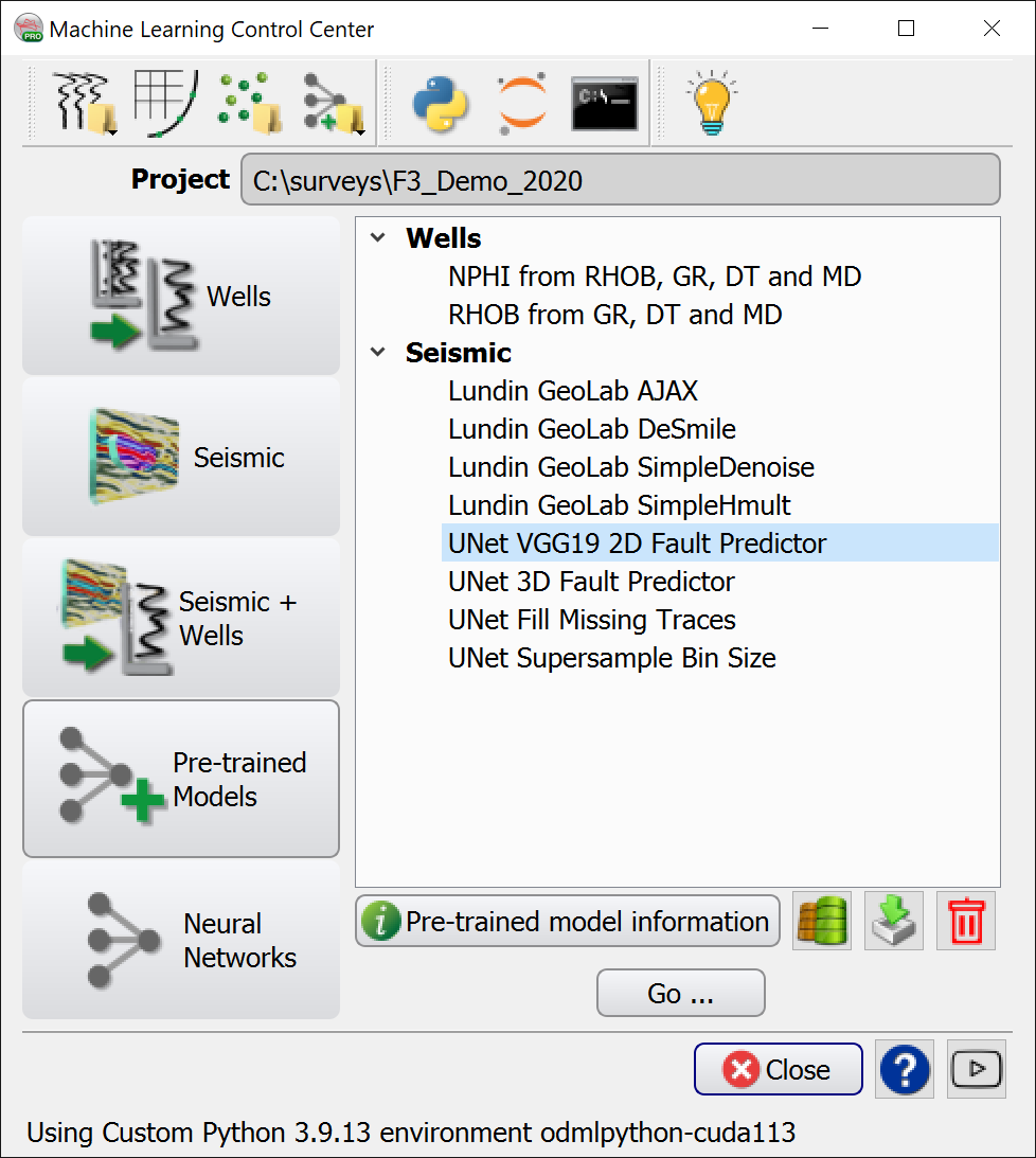
To use this pre-trained model, select the Unet 3D Fault Predictor and press Go.
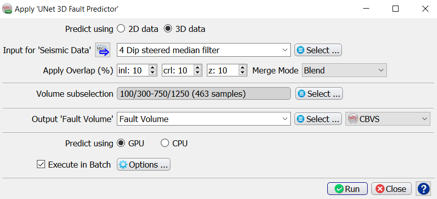
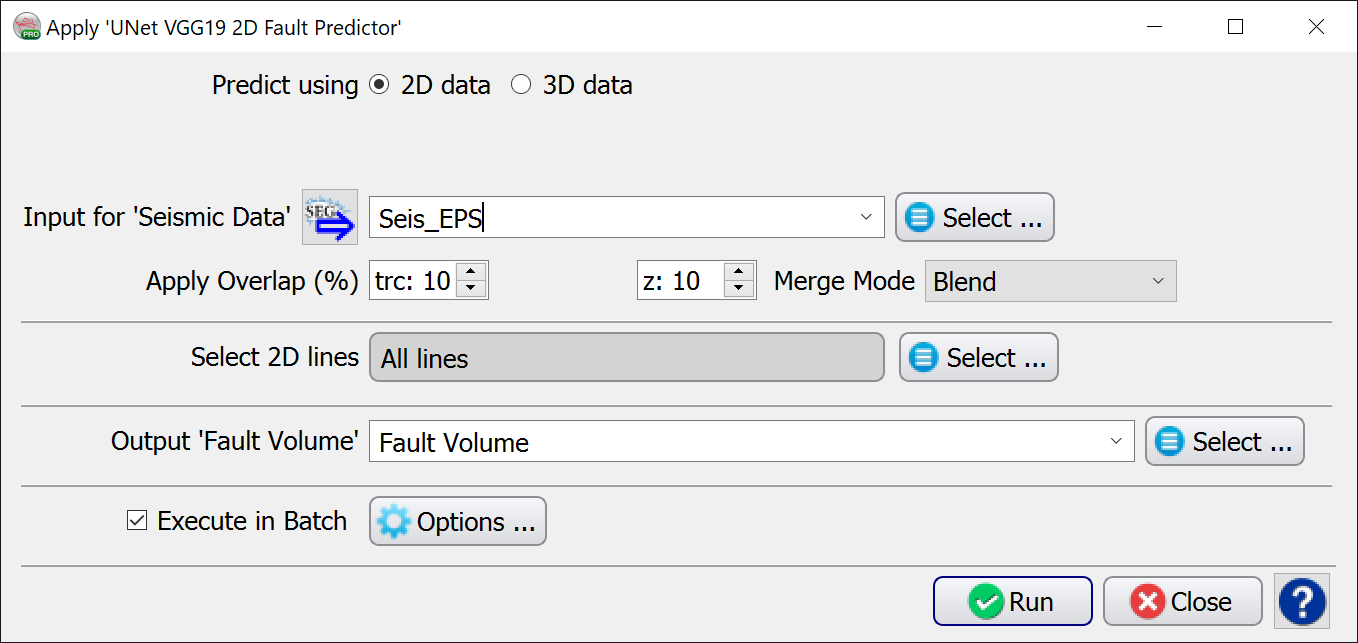
The Apply window pops up. Select the Input (Seismic Data) volume. The Overlap % is the percentage of overlap in Inline, Crossline and Z ranges of the images that are passed through the model. Optionally you can apply the trained model to a Volume subselection. Specify the output name of the Fault “Probability” Volume.
Predict using GPU is the default because this is much faster than predicting using CPU. Switch the toggle off if you do not have sufficient GPU memory to use this mode.
We do recommend enhancing the seismic before applying the Unet. Users can choose to remove any undesired noise from their seismic data by either using our dip steering median filter or the edge preserving filter which is part of the fault and fracture plugin.
The input cube is the seismic amplitude volume with 128x128x128 dimension in the inline/crossline/Z directions and the output will be a fault probability volume. Results of the Unet can be thinned in OpendTect by applying the Skeletonization (thinning algorithm).
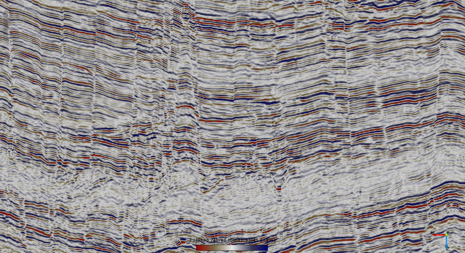
Figure 1. Original seismic (above).
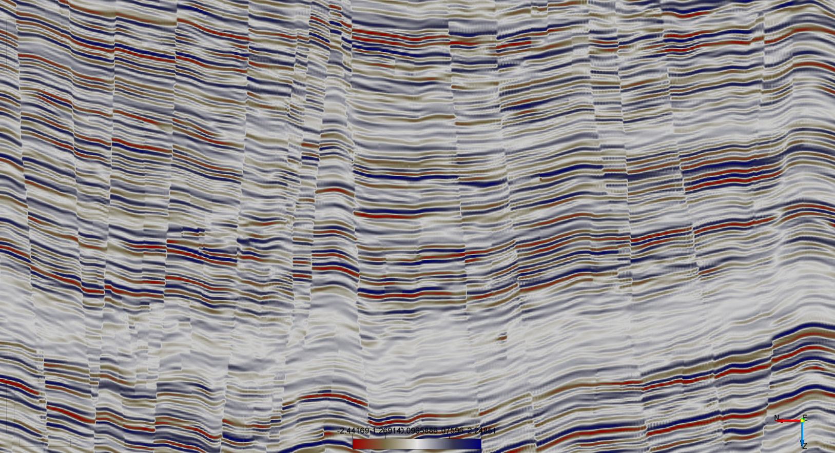
Figure 2. Seismic section after applying Edge Preserving Smoother (EPS).
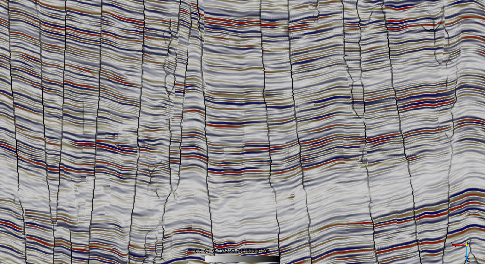
Figure 3. Results of the Unet Fault Predictor after applying the thinning. Faults are clearly imaged on both section and time slice.
For a different angle on the results, the image below is taken from an unthinned Fault Probability cube generated in this way.
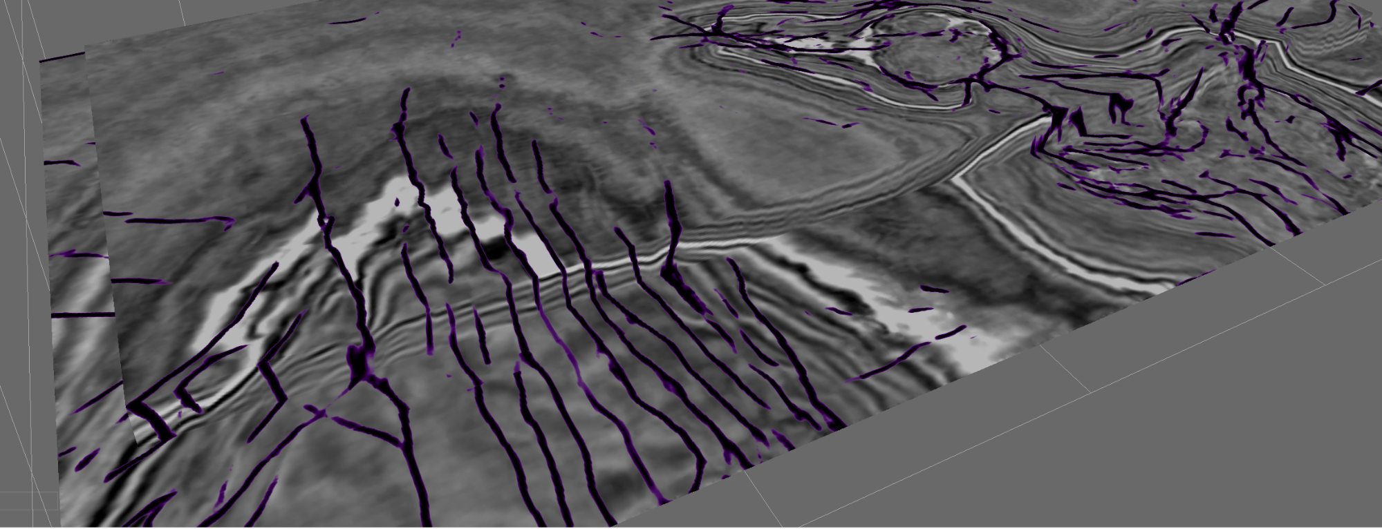
Figure 4: Output of the Unet 3D Fault Predictor on F3 Demo.
Reference: Wu, X, Liang, L., Shi, Y. and Fomel, S. [2019] FaultSeg3D: Using synthetic data sets to train an end-to-end convolutional neural network for 3D seismic fault segmentation. GEOPHYSICS, Vol. 84, No. 3 (May-June 2019); P. IM35–IM45, 11 FIGS. 10.1190/GEO2018-0646.1
Seismic - UNet VGG19 2D Fault Predictor
Predict Fault Likelihood from 2D seismic
2D U-Net VGG19 is an auto-encoder model that shares similarities with dGB's 2D U-Net. However, compared to the standard 2D U-Net, 2D U-Net VGG19 offers several advantages. By incorporating the VGG19 backbone, it can capture more complex and abstract features from the input data. This makes it better suited for transfer-training (tuning to a particular data set) than the standard 2D U-Net. Fault Likelihood range 0 to 1. It works best on Edge Preserving Smoothed data.
This model was trained on thousands of non-seismic images. In this model, we utilized the VGG19 model as our transfer learning model. The VGG19 model was the winning model in the ImageNet Large Scale Visual Recognition Challenge (ILSVRC) [Simonyan and Zisserman, 2015]. The VGG19 model have been trained using a large dataset of images called ImageNet. ImageNet is an open dataset that contains a wide range of natural images. It consists of 1000 image categories that are unrelated to seismic faults, such as candles, oysters, airliners, cats, cars, and more [see Russakovsky et al., 2015].
Next, this model was transfer-trained by dGB on synthetic seismic / fault images. Within the implementation of OpendTect's 2D VGG19, we extracted the pre-trained weights from the VGG19 model. These weights, representing the knowledge and patterns learned from ImageNet, were then transferred and applied to our fault predictor model. By leveraging the pre-existing knowledge encoded in the VGG19 weights, we accelerated the training process and enhanced the fault detection capabilities of our model. To facilitate the training process specifically for seismic fault prediction, we utilized Wu's synthetic fault seismic dataset [Wu et al., 2019].
This model can also be adjusted to work with real data by further training it (transfer-training) on interpreted sections. This means that we can fine-tune the model using actual seismic data, which improves its ability to detect faults in real seismic data [OpendTect Webinars: Building and Training Your 2D CNN Model with OpendTect, Applying and Fine-tuning your Trained Model: From U-Net Architecture to Real Seismic Data Interpretation].
Reference: A. Nawaz, U. Akram, A. A. Salam, A. R. Ali, A. Ur Rehman and J. Zeb, "VGG-UNET for Brain Tumor Segmentation and Ensemble Model for Survival Prediction," 2021 International Conference on Robotics and Automation in Industry (ICRAI), Rawalpindi, Pakistan, 2021, pp. 1-6, doi: 10.1109/ICRAI54018.2021.9651367.
Seismic - UNet Fill Missing Traces
Fill in missing traces in seismic.
Gaps of up to 10 traces can be filled. Output may need to be scaled post-application. Model has proved to work on an offshore data set with different geology, acquisition and processing located hundreds of kms away. It also worked to infill V-shape acquisition gaps in the shallow section of a nearby dataset.
The workflow to create this model is available as a Machine Learning Exercise from the Machine Learning Knowledge Base.
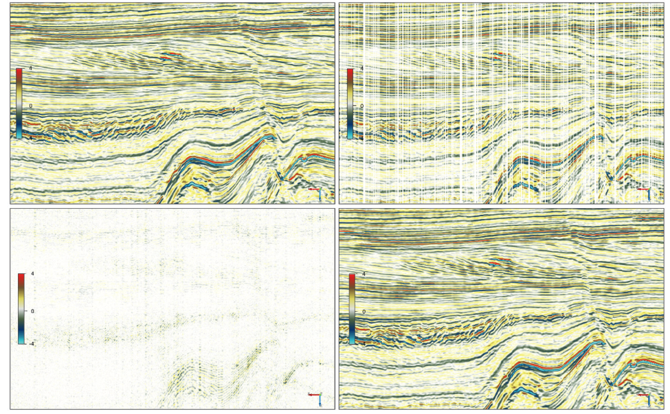
Example of Seismic crossline from F3 offshore The Netherlands. Clockwise from top-left: Input seismic; seismic with 33% randomly blanked traces; Machine learning reconstructed section; Difference between ground truth (upper-left) and machine learning reconstructed data (lower-right). All data is displayed after whole trace RMS scaling.
Reference: De Groot, P. and van Hout, M. [2021]. Filling gaps, replacing bad data zones and super-sampling of 3D seismic volumes through Machine Learning. EAGE Annual Conference & Exhibition, Amsterdam, 18-21 Oct. 2021.
Seismic - UNet Supersample Bin Size
Create a seismic data set with two times the number of traces in the inline and crossline directions.
To apply this model, you first need to create a new survey with an inline, crossline grid that has twice the number of traces as the original survey. You import the seismic data into this survey and use the tools in OpendTect (attribute engine and volume builder) to create a seismic volume with alternating live traces and traces with hard zeros in both inline and crossline direction. The output may need to be scaled post-application. Model has proved to work on an offshore data set with different geology, acquisition and processing located hundreds of kms away.
Seismic - Lundin GeoLab AJAX
Attenuate frequency dependent structurally consistent noise, enhance S/N and bandwidth for better interpretability.
AJAX is a model trained to do a series of postprocessing steps in order to enhance the visual quality and interpretability of a seismic volume. This includes (1) Frequency dependent structurally consistent noise attenuation and (2) Bandwidth enhancement. The model does not preserve amplitudes and frequency content of input volume.
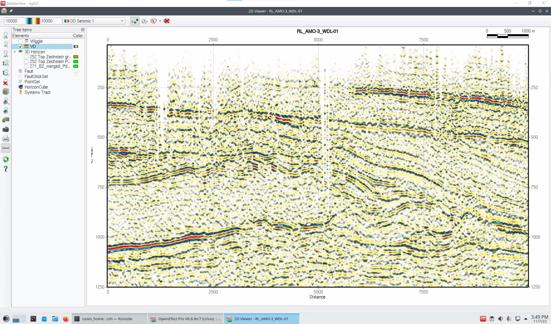
Before – AJAX Frequency dependent structurally consistent noise attenuation and bandwidth enhancement
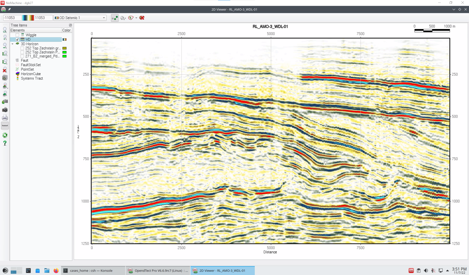
After - AJAX Frequency dependent structurally consistent noise attenuation and bandwidth enhancement
Seismic - Lundin GeoLab DeSmile
Attenuates migration smiles/artifacts and dip noise.
The migration of seismic data often causes moveout artifacts (smiles) that occur on seismic crosslines in final production volumes due to the sparse sampling in the crossline direction compared to the inline sampling. This model is trained to remove these artifacts and other dipping noise.
Suggestion: apply only in focus area where artifacts and dip noise is present to avoid affecting dipping primaries.
Before - DeSmile Attenuates migration smiles
After – DeSmile Attenuates migration smiles
Seismic - Lundin GeoLab SimpleDenoise
Attenuates random noise and jitter.
This model strictly attenuates noise (“salt & pepper”/jitter). Hence, both amplitudes and frequency of the primaries should be preserved.
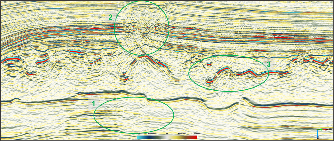
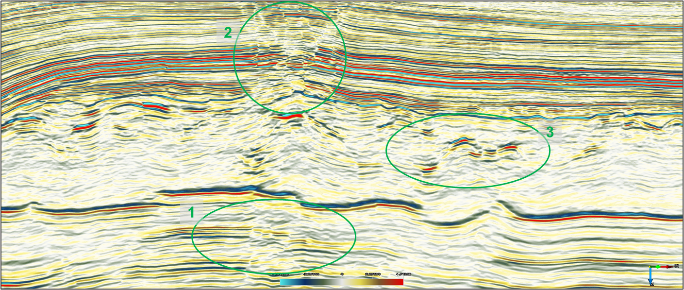
Seismic - Lundin GeoLab SimpleHmult
Attenuates horizon-parallel multiples.
This model removes horizon-parallel multiples (flat multiples). It is to be used to remove either seabed multiples, or other targeted multiples after flattening on target horizon. Should be applied only in window of interest to avoid removing too much primary energy elsewhere. Additional use: a tool to play with in order to understand the originator of the multiples.
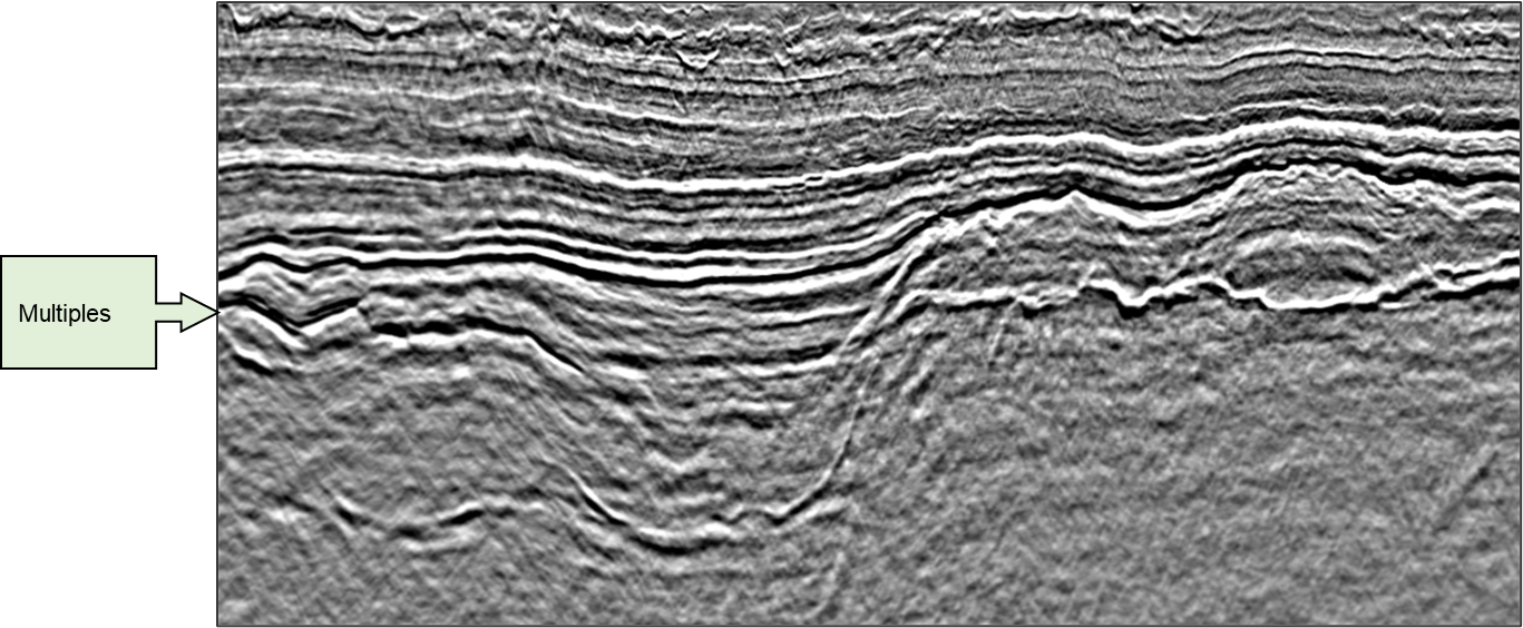
Before – SimpleHmult Attenuates horizon-parallel multiples
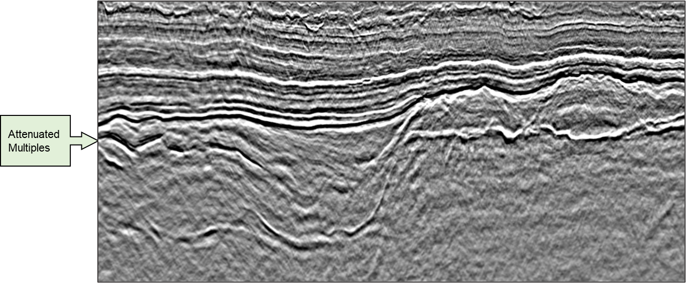
After - SimpleHmult Attenuates horizon-parallel multiples
Wells – NPHI from RHOB, GR, DT, and MD
Predict missing Neutron Porosity log from other input logs.
This example is a log-log prediction. The XGBoost model in this example learned to predict NPHI logs from DT, RhoB, GR and MD curves. The training set consists of 219 wells from the Dutch North Sea.
Works best when all input logs are present in the interval of application.
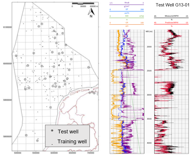
Results of the trained model on well G13-01, a well from the validation set.
XGBoost prediction of NPHI from GR, DT, RhoB and MD in G13-01, a blind test well. The correlation coefficient between measured NPHI (black) and predicted NPHI (red) is 0.93 for the entire validation set of 36 wells and 0.96 for this well.