3.5 Seismic + Wells models
The aim of seismic + wells workflows is to predict a well log property from seismic input features. Input and target can either come from real wells and real seismic features (e.g. elastic impedance data) or from synthetic data created by SynthRock.
We will explain the user interface on the basis of a simple example in which we create a Porosity volume from an inverted Acoustic Impedance volume.
Please note that the current implementation of this workflow only accepts input features from the seismic side (most often in Two-Way-Time) while target features are extracted from well logs (in depth). This is not desirable because to extract matching inputs and targets the well ties must be perfect. This is never the case. As we only need to find a relationship between Acoustic Impedance and Porosity it makes sense to extract both inputs and targets from logs. In this case: Acoustic Impedance logs and corresponding Porosity logs. This ensures alignment over the entire well track. Application of this relationship (the trained model) will transform the AI volume to a Porosity volume with the same mis-ties inherent in the AI volume.
The workflow described above will be implemented in the near future. Training data can then be extracted from real wells and from pseudo-wells created with SynthRock. The workflow can already be emulated in OpendTect albeit a bit cumbersome. It requires a few extra data preparation steps: use the LogCube option to convert the input AI logs to pseudo-seismic cubes at 4ms sampling (you can even use and create extra attribute cubes from them like log of AI, sqrt of AI, derivative of AI with depth etc. to have more input features). Before using these cubes to predict porosity in the Seismic+Wells UI, you might want to apply a low pass filter to have them at the same frequency as the inverted AI.
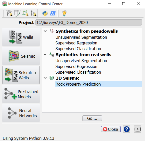
Let’s follow the workflow as implemented in the current release without such preprocessing steps. We have 4 wells with Porosity logs. Select the workflow and press Go.
Extract Data
Input Data
In the Input Data tab of the ‘Property Prediction’ Window, Select the input feature(s). In this case only one volume is selected: the Acoustic Impedance Cube with name “7a AI Cube std”.
Select the Target Log. In this demo exercise we select all four wells for training. In a real study we recommend reserving at least one well as blind test well (Validation Set).
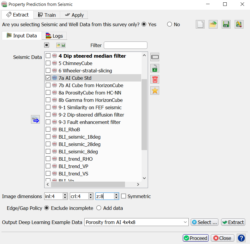
The Image dimensions specify how many traces in inline and crossline steps around the well track will be extracted. The Image dimensions in inline and crossline directions multiply our examples. Each example has slightly different seismic characteristics but the target porosity value at each position along the track is the same.
The Edge/Gap Policy controls how we handle examples with missing input features. With a Stepout of 10 we need 10 samples above and 10 samples below each prediction point. The default Exclude incomplete will not return a value meaning we lose 10 samples above and 10 samples below each gap. If the toggle is set to Add data, the value at the edge of an input feature is copied Stepout times to ensure the model can make a prediction at the edge. In other words the predicted log covers the same interval as the input logs (gaps do not increase).
Log Tab
In the Log tab, select the Target Logs. In this exercise select all four wells for training. In a real study we recommend reserving at least one well as blind test well (Validation Set). Then press OK.
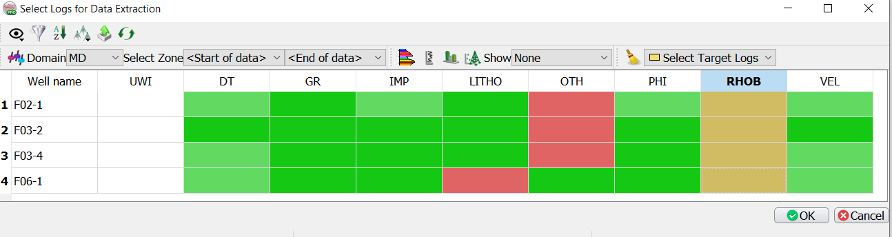

To extract only in a zone of interest, we can select the corresponding markers to Extract between a pair of specified start and end points. If left to defaults, the entire log will be used.
The Extra Z above/below (ms) depends on the velocity. We have seismic in TWT and logs in depth. We want to have roughly the same sampling rates for both (we can ensure this, as well as perfect alignment if we use the LogCube preprocessing steps explained above).
The selection can be Saved, retrieved (Open) and Removed using the corresponding icons.
Specify an output name for the Deep Learning Example Data (the Training Set) and press Extract.
Press Proceed to continue to the Training tab.
Training
When we already have stored the extracted data for training, we can move on to the Training tab with Select training data (Input Deep Learning Example data). After the training data is selected the UI shows which models are available.
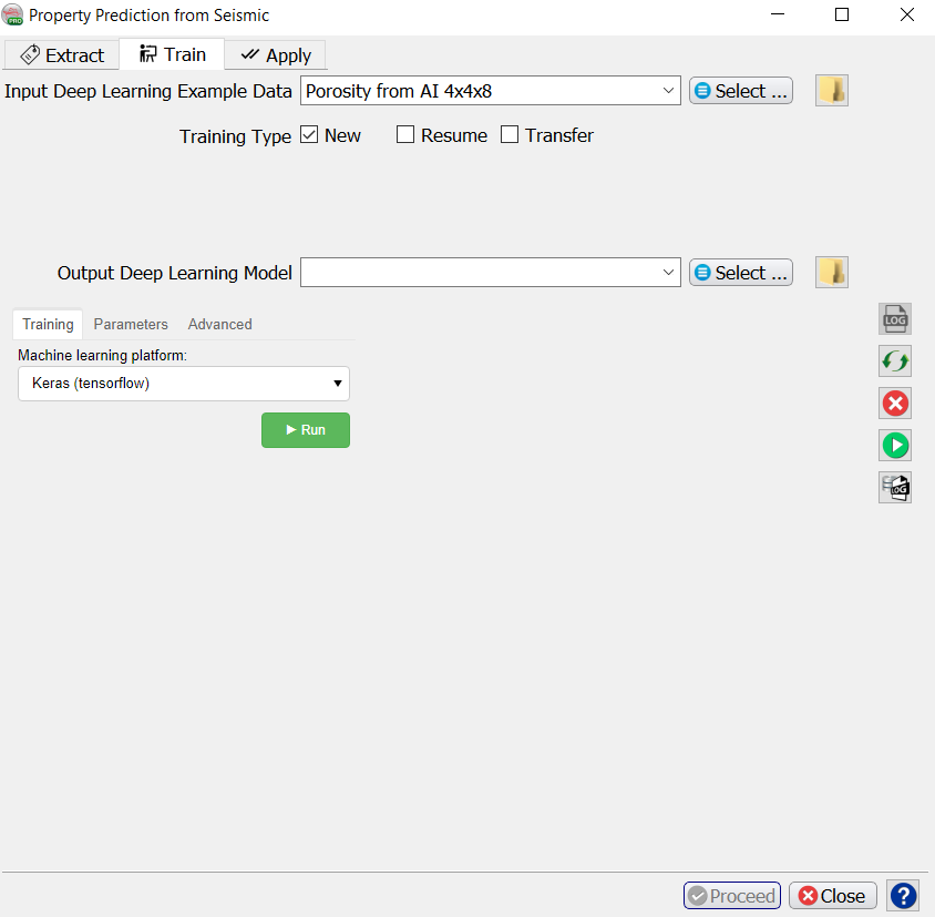
Under the Select training data there are three toggles controlling the Training Type:
- New starts from a randomized initial state.
- Resume starts from a saved (partly trained) network. This is used to continue training if the network has not fully converged yet.
- Transfer starts from a trained network that is offered new training data. Weights attached to Convolutional Layers are not updated in transfer training. Only weights attached to the last layer (typically a Dense layer) are updated.
The supported models are divided over three platforms: Scikit Learn, PyTorch and Keras (TensorFlow).
Check the Parameters tab to see which models are supported and which parameters can be changed. From Scikit Learn we currently support:
- Linear Regression
- Ordinary Least Squares
- Ensemble Methods
- Random Forests
- Gradient Boosting
- Adaboost
- XGBoost
- Neural Networks
- Multi-Layer-Perceptrons
- Support Vector Machines
- Linear
- Polynomial
- Radial Basis Function
- Sigmoid
Our best results have been generated with Random Forests and XGBoost (eXtreme Gradient Boosting of Random Forest Models). Random Forests build a bunch of trees at once and average the results out at the end, while gradient boosting generates and adds one tree at a time. Because of this gradient boosting is more difficult for parameter tuning, but since it goes more in depth, it could result in higher accuracy for complicated or imbalanced datasets.
From a statistics point of view, a Random Forest is a 'bagging' algorithm, meaning that it combines several high variance, low-bias individual models to improve overall performance. Gradient boosting is a 'boosting' algorithm, meaning that it combines several high-bias, low variance individual models to improve overall performance. For parameter details we refer to the Scikit Learn User Guide.

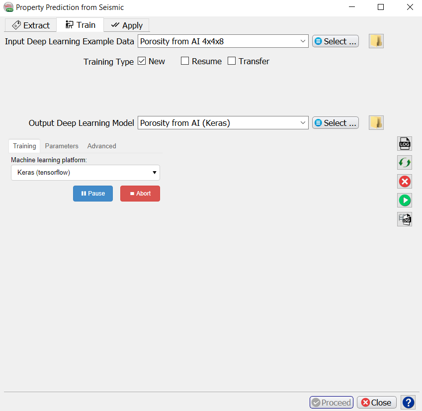
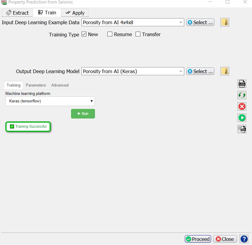
After model selection, return to the Training tab, specify the Output Deep Learning model and press the green Run button. This starts the model training. In this tab, the Run button is now replaced by Pause and Abort buttons.
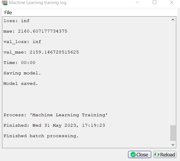
The progress can be followed in a text log file. If this log file does not start automatically, please press the log file icon in the toolbar on the right-hand side of the window.
Below the log file icon there is a Reset button to reload the window. Below this there are three additional icons that control the Bokeh server, which controls the communication with the Python side of the Machine Learning plugin. The server should start automatically. In case of problems it can be controlled manually via the Start and Stop icons in the side ribbon. The current status of the Bokeh server can be checked by viewing the Bokeh server log file.
When the processing log file shows “Finished batch processing”, you can move to the Apply tab.
The following section describing training of a Keras model is given for completion's sake.
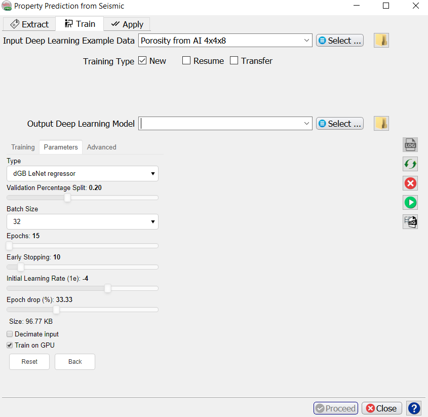
The dGB LeNet regressor is a fairly standard Convolutional Neural Network that is based on the well-known LeNet architecture (and available in Keras-TensorFlow) It should be noted that satisfactory seismic-log prediction results have not been generated with this model. It is included here to give researchers a starting point for seismic-log prediction with Keras / TensorFlow models. We encourage workers to use this model as a starting point, and perhaps find a better one (that we will gladly add to the list of supported models).
The following training parameters can be set:
Batch Size: this is the number of examples that are passed through the network after which the model weights are updated. This value should be set as high as possible to increase the representativeness of the samples on which the gradient is computed, but low enough to have all these samples fit within the memory of the training device (much smaller for the GPU than the CPU). If we run out of memory (raises a Python OutOfMemory exception), lower the batch size!
Note that if the model upscales the samples by a factor 1000 for instance on any layer of the model, the memory requirements will be upscaled too. Hence a typical 3D Unet model of size 128x128x128 will consume up to 8GB of (CPU or GPU) RAM.
Epochs: this is the number of update cycles through the entire training set. The number of epochs to use depends on the complexity of the problem. Relatively simple CNN networks may converge in 3 epochs. More complex networks may need 30 epochs, or even hundreds of epochs. Note, that training can be done in steps. Saved networks can be trained further when you toggle Resume.
Early Stopping: this parameter controls early stopping when the model does not change anymore. Increase the value to avoid early stopping.
Initial Learning rate: this parameter controls how fast the weights are updated. Too low means the network may not train; too high means the network may overshoot and not find the global minimum.
Epoch drop: controls how the learning rate decays over time.
Decimate Input: This parameter is useful when we run into memory problems. If we decimate the input the program will divide the training examples in chunks using random selection. The training is then run over chunks per epoch meaning the model will eventually have seen all samples once within one epoch, but only no more than one chunk of samples will be loaded in RAM while the training is performed.
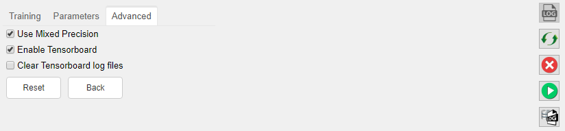
Mixed precision: Mixed precision option has been added to dgbpy for both PyTorch and Keras platform. This allows to train models using a combination of 16-bit and 32-bit precision formats which will optimize GPU memory usage and efficiency. The GPU memory usage can be reduced by 50% and 75% in some cases. It also increases training speed 2 - 3 times on GPUs with Volta or Turing architectures. This doesn't also affect training accuracy or performance.
For more details about what is ‘Mixed precision training’ please refer to:
After model selection, return to the Training tab, specify the Output Deep Learning model and press the green Run button. This starts the model training. In this tab, the Run button is now replaced by Pause and Abort buttons.
The progress of Keras / TensorFlow runs can be monitored using TensorBoard, which automatically starts up in your default browser. Please note that it may take a few minutes before TensorBoard has gathered enough information to present training progress charts. It is recommended to clear the TensorBoard log files from time to time using Clear TensorBoard log files as all TensorBoard information is retrieved for all current and historic runs.
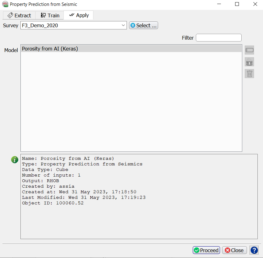
Apply
In the “Property Prediction from Seismic” window, select the trained model and press Proceed.

Select the Input Cube, optionally specify a Volume subselection and give an output name for the seismic Output volume. Press Run. This will start a batch job. Progress can be monitored in the log file that is automatically launched.