3.4.2 Seismic Classification (Supervised 2D and 3D)
This workflow maps a seismic image (1D, 2D, or 3D) to a single point that represents a certain class. This is a supervised method in which the user provides the desired output in the form of a set of pointsets. Each pointset represents a different class. Application of the trained model delivers a classification cube (or 2D line set).
We will discuss the workflow and UI on the basis of a 3D seismic classification into 9 different seismic facies classes. Each class represents a seismic class interpreted on one line. The pointsets for each case can be picked manually, or they can be created automatically using the tools in OpendTect (e.g. pointsets can be generated by sampling between mapped horizons, or by sampling inside interpreted 3D bodies).
In this case the point sets were copied from the MalenoV example by: Rutherford Ildstad, C., and Bormann, P., 2017. MalenoV: Tool for training and classifying SEGY seismic facies using deep neural networks: https://github.com/bolgebrygg/MalenoV.
Extract Data
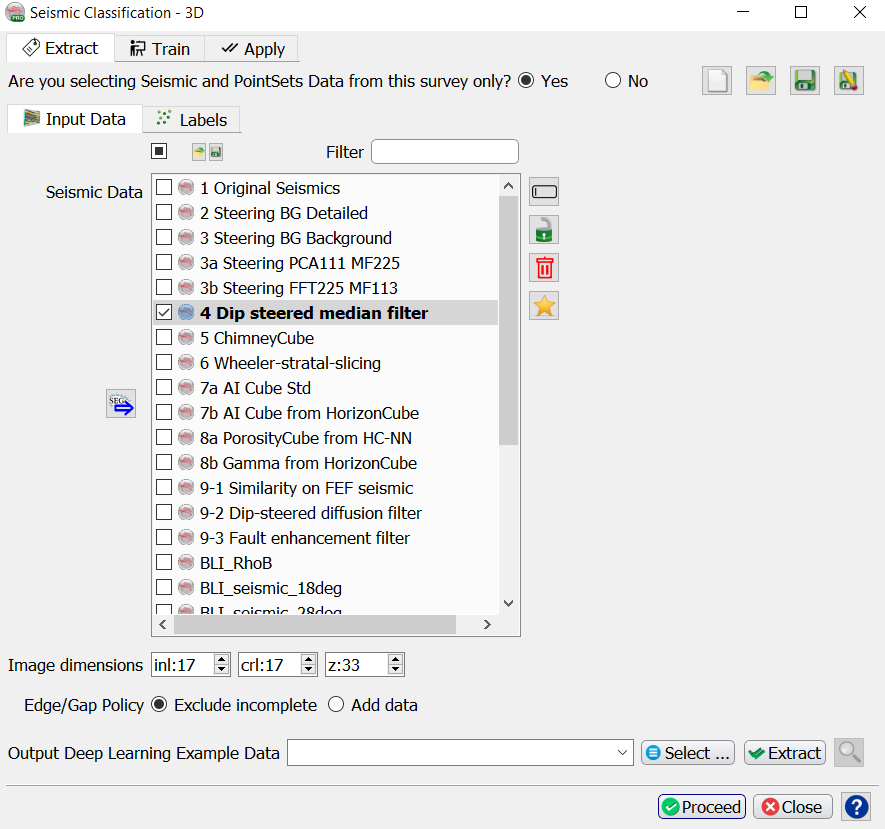
Input Data
Select the seismic data in the Input Data tab.
Image dimensions are the number of samples of the extracted cubelets.
Examples:
- Stepouts Inl: 8; Crl: 8, Z: 16 (number of samples on either side of the evaluation point) extracts cubelets of 17x17x33 samples.
- Stepouts Inl: 0; Crl: 16, Z: 8 extracts 2D images along inlines with dimensions 33x17 samples.
Edge/Gap policy determines how to treat incomplete examples. The default is to exclude incomplete data. Add data copies neighboring samples to complete the example.
Labels
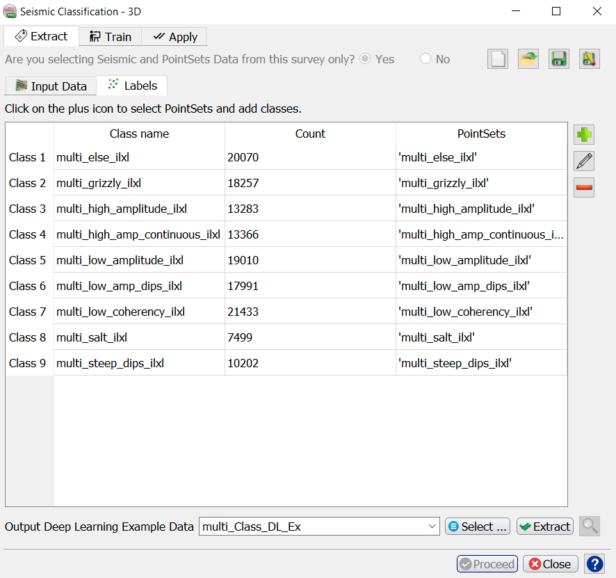
Select the PointSets and add classes in the Labels tab.
Press the Select button to start the extraction process for the input data.
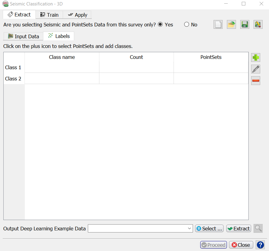
Press the + icon. This pops up the “Select PointSets” window.
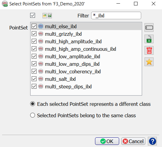
In this example select the nine PointSets ‘multi…_ilxl’. The model will be trained to classify the response into the numbers 1, 2, …, 8, 9.
When you have selected all point sets for one class press OK to return to the “Deep Learning Class Definition” window.
Repeat this process if you want to add more examples from other point sets. These point sets can be located in different surveys. For example, if you have created Chimney Cubes in the past and you saved the Chimney-Yes and Chimney-No point sets, you can re-use these to train a deep learning model on all these examples.
Repeat the process by pressing + until all examples for classes are defined.
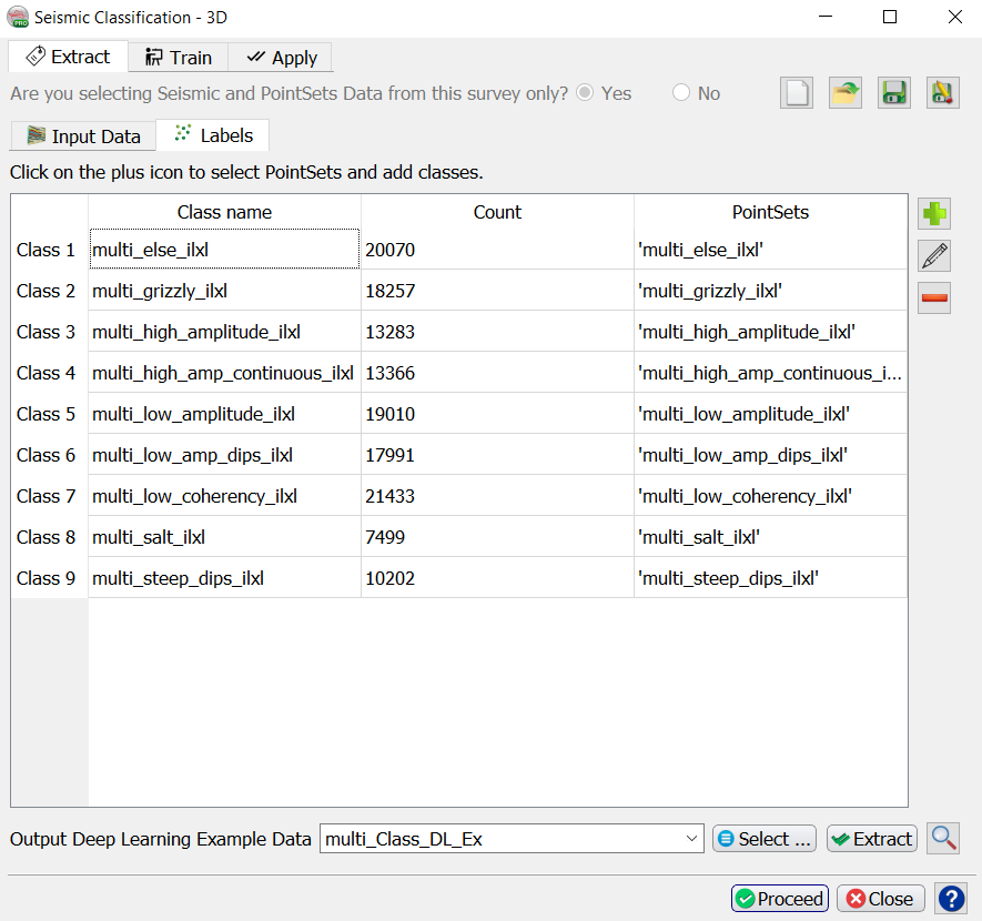
Specify the name of the Output Deep Learning Example Data and press Extract to start the extraction process.
When this process is finished you are back in the “Seismic Classification” start window. The Proceed button has turned green. Press it to continue to the Training tab.
Both the Class Examples and the Class Definition selections can be Saved, retrieved (Open) and modified (Edit) using the corresponding icons below the + icon. Remove deletes the respective selection file from the database.
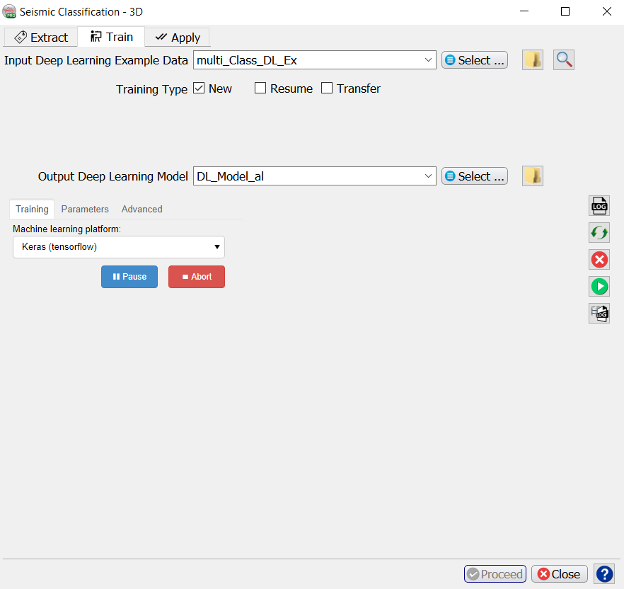
Training
When you already have stored data, you can start in the Training tab with Select training data (Input Deep Learning Example data).
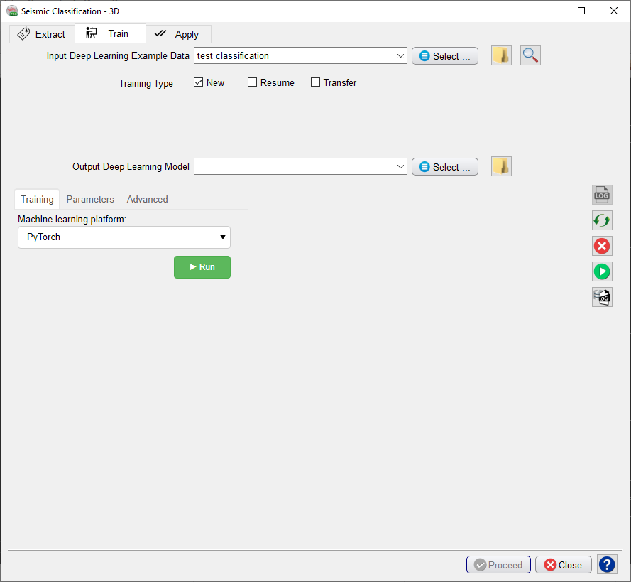
Under the Select training data there are three toggles controlling the Training Type:
- New starts from a randomized initial state.
- Resume starts from a saved (partly trained) network. This is used to continue training if the network has not fully converged yet.
- Transfer starts from a trained network that is offered new training data. Weights attached to Convolutional Layers are not updated in transfer training. Only weights attached to the last layer (typically a Dense layer) are updated.
After the training data is selected the UI shows which models are available. These models are divided over three platforms: Scikit Learn, PyTorch and Keras (TensorFlow).
Check the Parameters tab to see which models are supported and which parameters can be changed. From Scikit Learn we currently support:
For parameter details we refer to: the Scikit Learn User Guide.
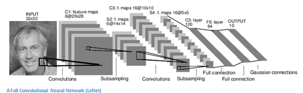
From Keras (TensorFlow) we currently support the classic LeNet Convolutional Neural Network for log-log prediction.
The dGB LeNet regressor is a fairly standard Convolutional Neural Network that is based on the well-known LeNet architecture (below).
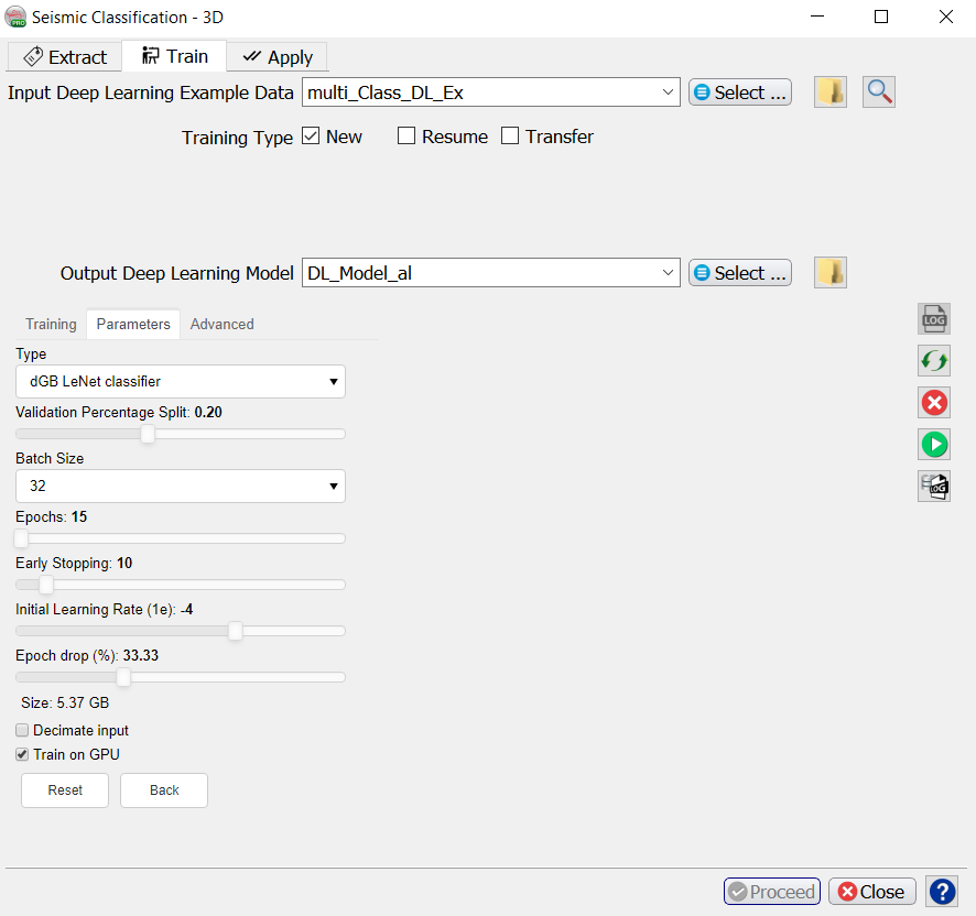
The following training parameters can be set in the Parameters tab:
Batch Size: this is the number of examples that are passed through the network after which the model weights are updated. This value should be set as high as possible to increase the representativeness of the samples on which the gradient is computed, but low enough to have all these samples fit within the memory of the training device (much smaller for the GPU than the CPU). If we run out of memory (raises a Python OutOfMemory exception), lower the batch size!
Note that if the model upscales the samples by a factor 1000 for instance on any layer of the model, the memory requirements will be upscaled too. Hence a typical 3D Unet model of size 128-128-128 will consume up to 8GB of (CPU or GPU) RAM.
Epochs: this is the number of update cycles through the entire training set. The number of epochs to use depends on the complexity of the problem. Relatively simple CNN networks may converge in 3 epochs. More complex networks may need 30 epochs, or even hundreds of epochs. Note, that training can be done in steps. Saved networks can be trained further when you toggle Resume.
Early Stopping: this parameter controls early stopping when the model does not change anymore. Increase the value to avoid early stopping.
Initial Learning rate: this parameter controls how fast the weights are updated. Too low means the network may not train; too high means the network may overshoot and not find the global minimum.
Epoch drop: controls how the learning rate decays over time.
Decimate Input: This parameter is useful when we run into memory problems. If we decimate the input the program will divide the training examples in chunks using random selection. The training is then run over chunks per epoch meaning the model will eventually have seen all samples once within one epoch, but only no more than one chunk of samples will be loaded in RAM while the training is performed.
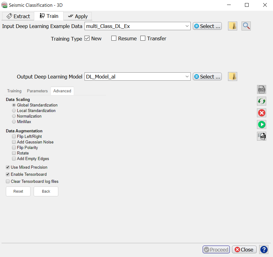
Mixed precision: Mixed precision option has been added to dgbpy for both PyTorch and Keras platform. This allows to train models using a combination of 16-bit and 32-bit precision formats which will optimize GPU memory usage and efficiency. The GPU memory usage can be reduced by 50% and 75% in some cases. It also increases training speed 2 - 3 times on GPUs with Volta or Turing architectures. This doesn't also affect training accuracy or performance.
For more details about what is ‘Mixed precision training’ please refer to:
After model selection, return to the Training tab, specify the Output Deep Learning model and press the green Run button. This starts the model training. The Run button is replaced in the UI by Pause and Abort buttons.
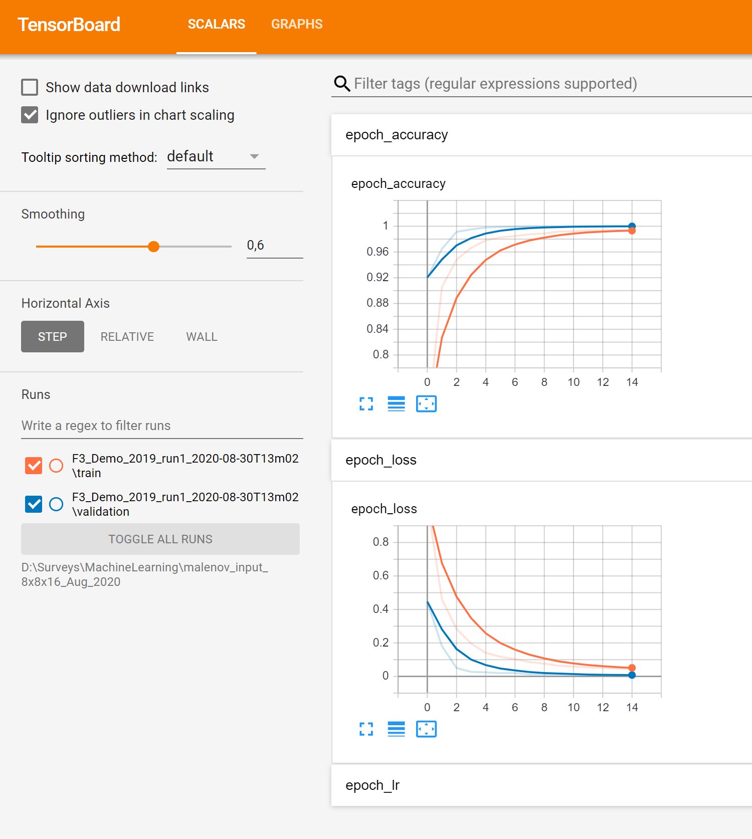
The progress of Keras / TensorFlow runs can be monitored in TensorBoard, which automatically starts up in your default browser. Please note that it may take a few minutes before TensorBoard has gathered the information that is gathered during training. As all TensorBoard information on your machine is retrieved for all current and historic runs it is recommended to clear the TensorBoard log files from time to time. You can do this with the Clear TensorBoard log files toggle in the Advanced parameters before any Run.
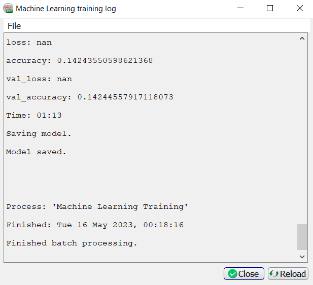
The progress can be also followed in a text log file. If this log file does not start automatically, please press the log file icon in the toolbar on the right-hand side of the window:
Below the log file icon there is a Reset button to reload the window. Below this there are three additional icons that control the Bokeh server, which controls the communication with the Python side of the Machine Learning plugin. The server should start automatically. In case of problems, it can be controlled manually via the Start and Stop icons. The current status of the Bokeh server can be checked by viewing the Bokeh server log file.
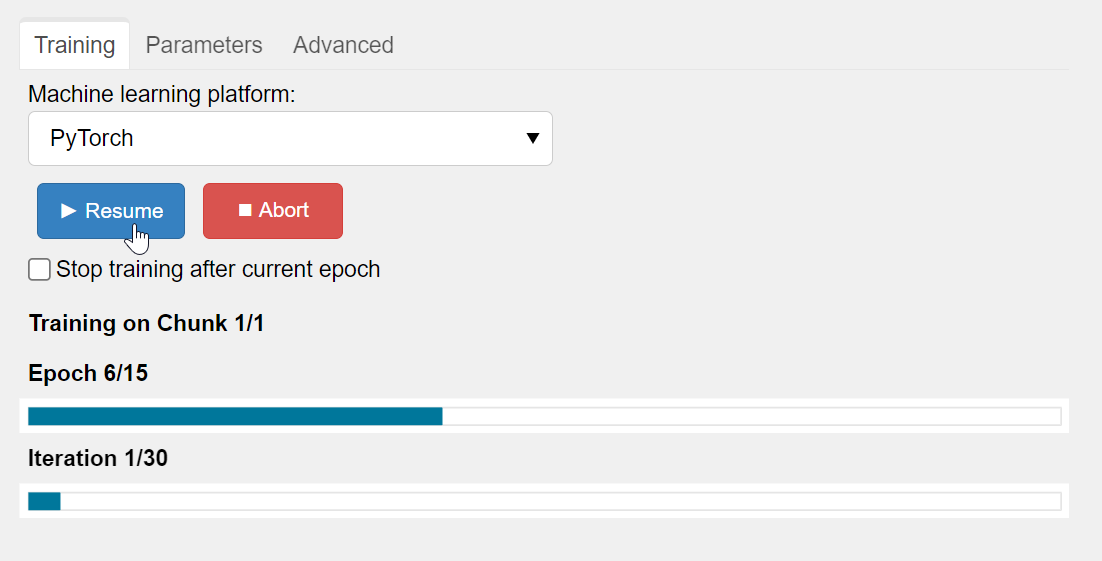
The user also has the opportunity to Pause or Abort the training for any reason. Depending on the platform chosen, there may also be the option to check the box to Stop training after the current epoch. If paused, then the user will be given the chance to Resume:
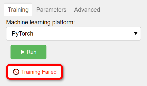
And choosing to Abort will immediately fail the training:
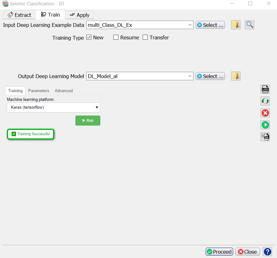
When the processing log file shows “Finished batch processing”, and the Training window shows “Training Successful’, you can move to the Apply tab.
Apply
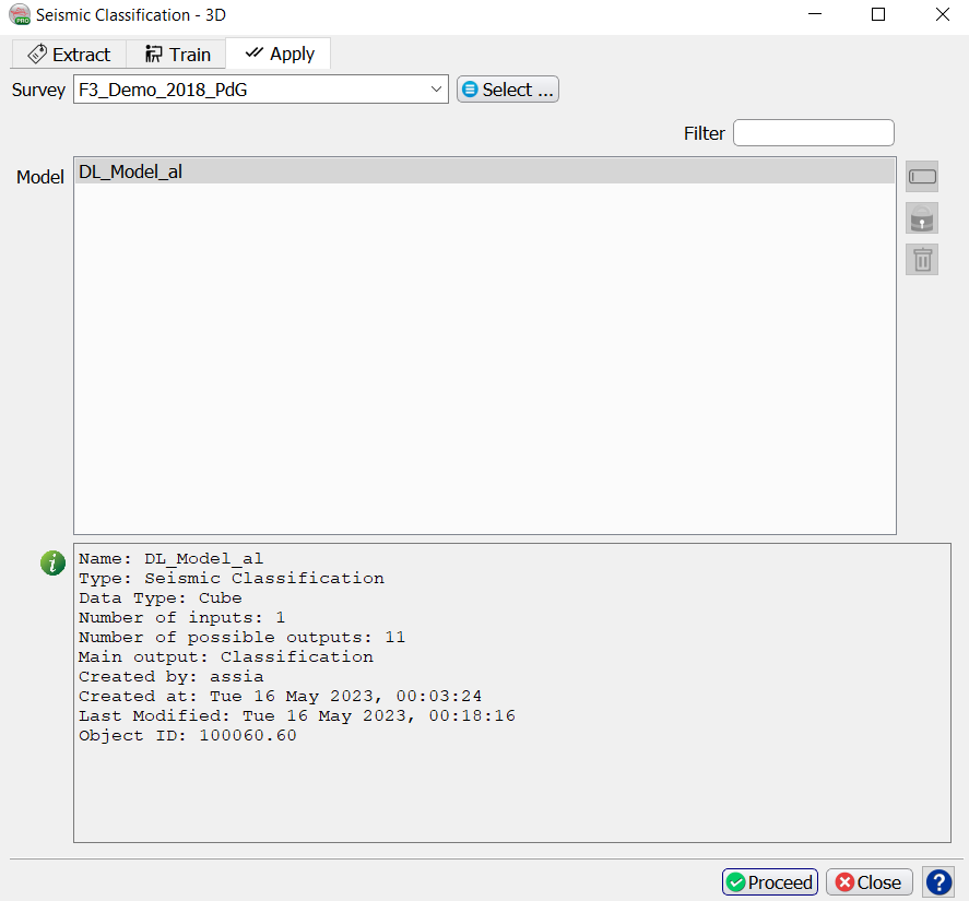
Once the Training is done, the trained model can be applied. Select the trained model and press Proceed.
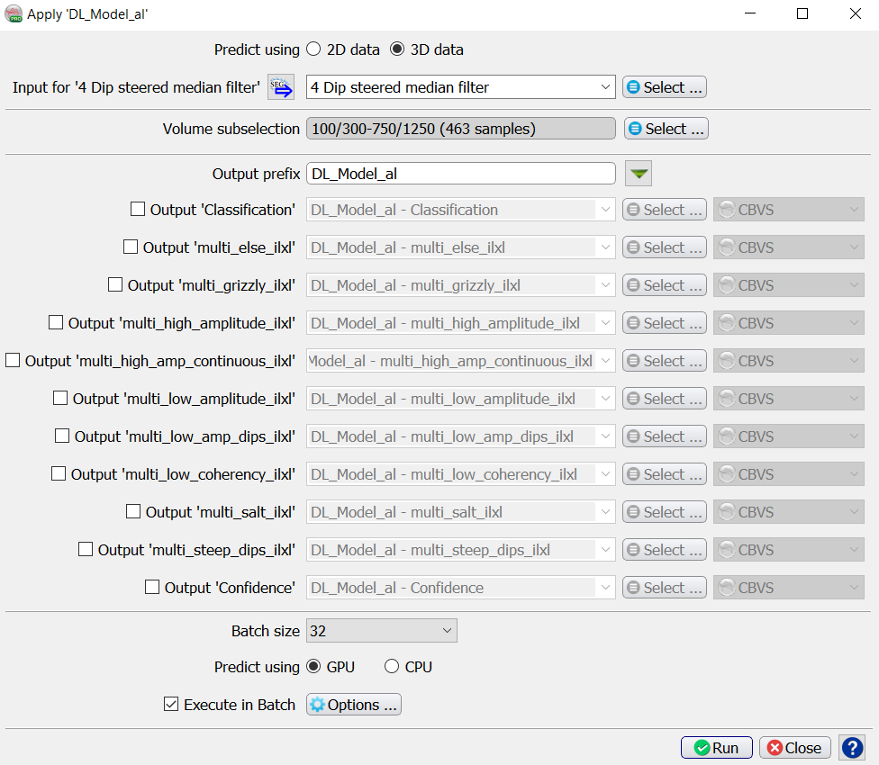
The Apply window pops up. Here you optionally apply to a Volume subselection. You can output a Classification Volume (values 1 to 9 in this case), a Confidence volume and Probability volumes for each of the output classes. Each output is stored in a separate cube in CBVS format, or SEGY format. The names of all outputs are given the same Output prefix. To change the prefix for all selected output cubes, press the funnel icon next to the prefix name.
Probability is simply the output of the prediction node which ranges between 0 and 1.
Confidence is computed as the value of the winning node minus the value of the second best node.
The Batch size is only important for the speed. If the batch size is set too high you may run out of memory (GPU or CPU depending on the Predict using GPU toggle). Running the application on a GPU is many times faster than running it on a CPU. Press Run to create the desired outputs. The image below is taken from a seismic facies Classification cube generated in this way.
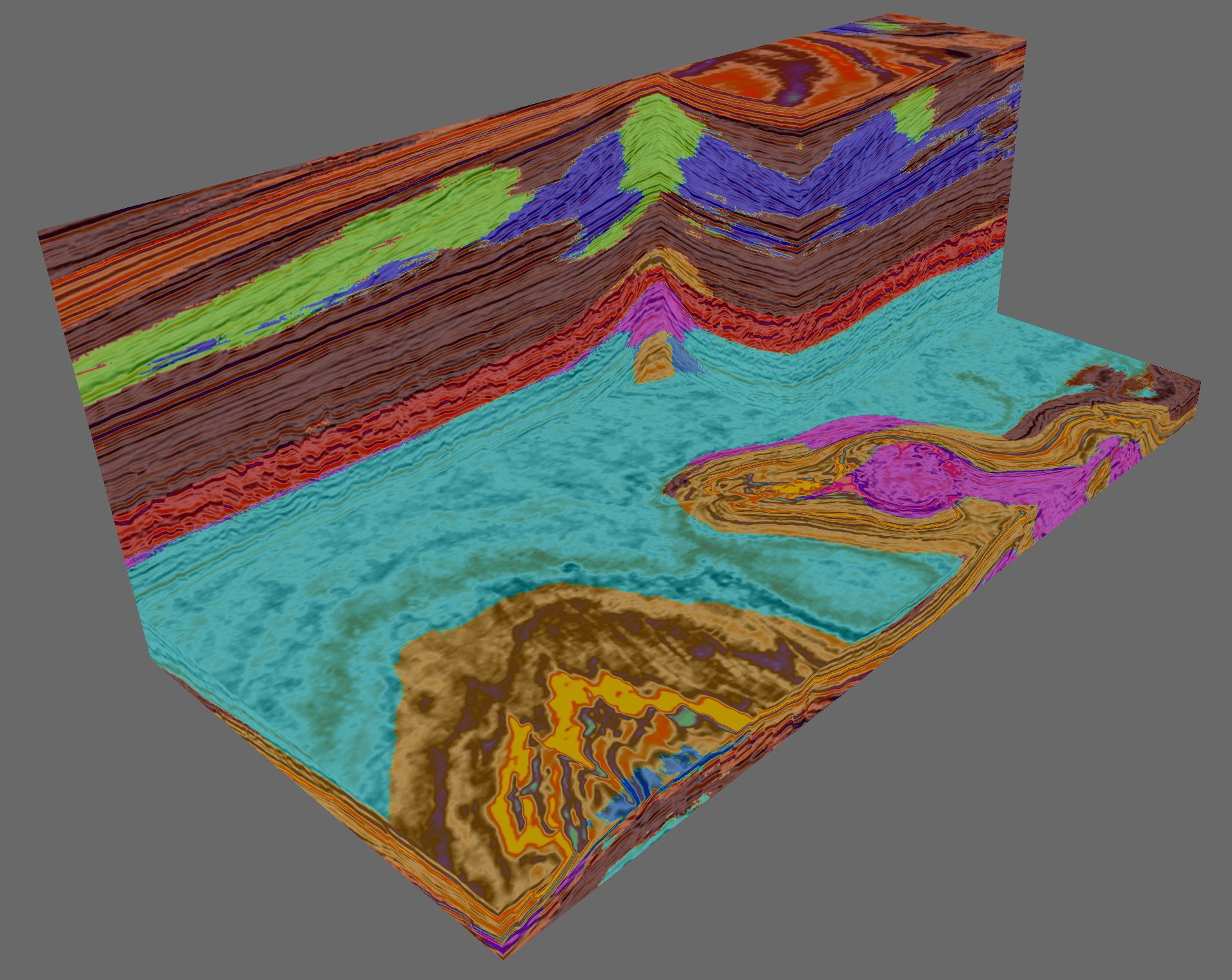
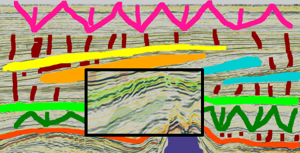
Output of the trained model: seismic facies cube.