3.4.3 Seismic Image Segmentation (Supervised 2D and 3D)

A Segmentation model maps a seismic image (1D, 2D, or 3D) to a labelled image (mask) of similar size where the output has discrete values (0 or 1, or 1, 2, …, N).

These workflows are categorized as supervised methods in that the input data set(s) and the target data are provided to facilitate training. For example, if you have a 3D seismic volume and a target 3D volume with values 1 at fault planes and 0 elsewhere, you can extract (2D images or 3D cubelets) from both volumes to create a model for fault prediction. Application of the trained model delivers a segmentation volume (3D seismic) or a line set (2D seismic). We will discuss the workflow and user interface components on the basis of a 3D example.

The objective is to predict geologically meaningful layers from seismic input. We will train a Unet on 2 input features:

1. 2D synthetic seismic images (128 x 128 samples)

2. 2D images of Two-Way-Time (TWT also of 128 x 128 samples)

 

The desired output are 2D images (128 x 128 samples) containing labels (1 to 8). The reason for using TWT in addition to the seismic input feature is to help the model find the logical order in the segments (layers are stacked: 1 is on top; 8 is the lowest). The trained Unet is applied to real 3D data. The output is a 3D segmented volume. If successful, this workflow can be applied to quickly segment unseen seismic volumes with similar geology. The Figure below shows the synthetic data.

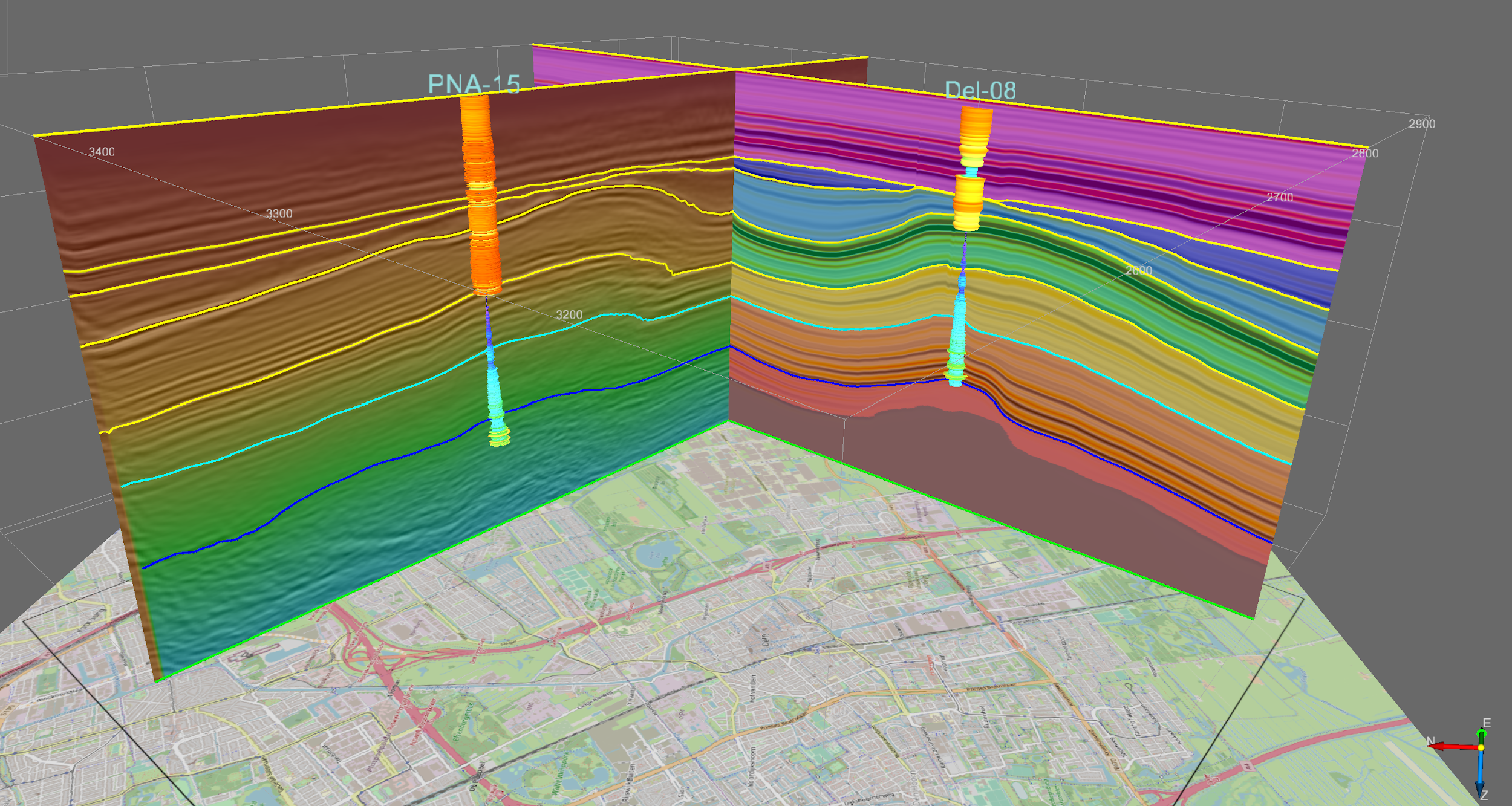
Synthetic data over the city of Delft. The synthetic data set was created in OpendTect from a set of interpreted 3D horizons and 2 wells with Acoustic Impedance logs. The logs were interpolated in the Volume Builder. The synthetic seismic volume, interval labels volume (mask) and Two-Way-Time volume were created in the attribute engine. Seismic inline through DEL-08 shows synthetic seismic co-rendered with target labels. Seismic crossline through PNA-15 shows synthetic seismic co-rendered with Two-way time.

 

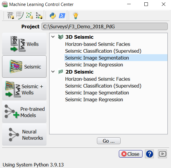
Select the Seismic Image Segmentation workflow and press Go.

 

Extract Data

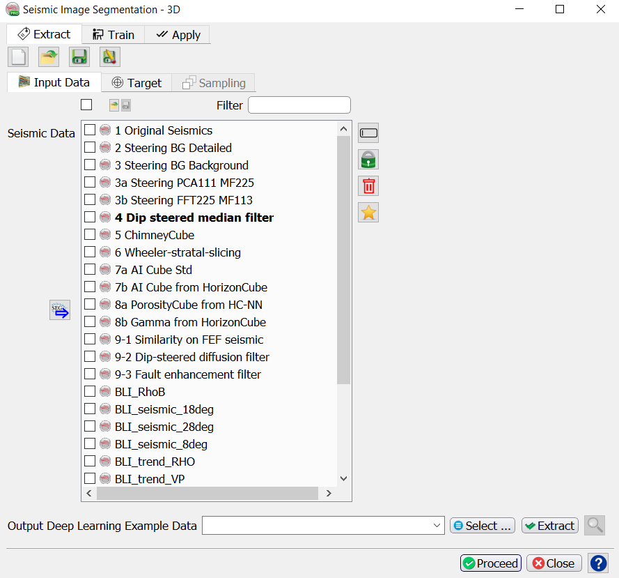
Input Data tab, select the input seismic data for prediction.

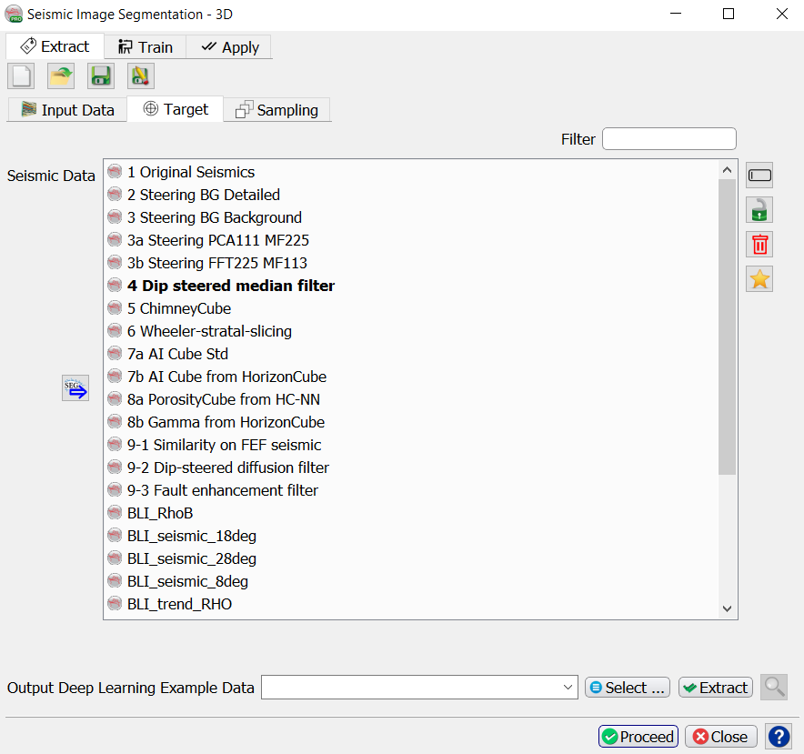
Target tab, select the target seismic volume containing the labels. In the example this volume is called “classification”.

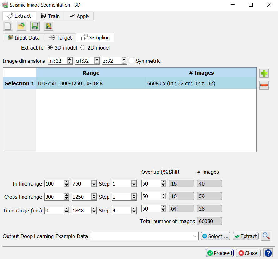
Sampling tab, select the image dimensions of the input features.

Image Dimensions are the number of samples in inline, crossline and Z directions.

Examples:

• Inl: 0; Crl: 128, Z: 128 - extracts 2D images along inlines with dimensions 128 x 128 samples
• Inl: 64, Crl: 64, Z: 64 - extracts cubelets of 64x64x64 samples.

The examples (images) are extracted from the specified Inline, Crossline and Time Ranges. Step is the sampling rate in the bin (time) directions. The Overlap determines how much overlap there is between neighboring images. The total number of images is given on the right-hand side of the window. You can control this number by playing with the ranges and overlap parameters.

Different seismic selections can be used by pressing the + icon.

The Seismic Image Segmentation Parameters can be Saved, retrieved (Open) and Deleted using the corresponding icons.

Specify the name of the Output Deep Learning Example Data and press Extract to start the extraction process.

When this process is finished the Proceed button has turned green. Press it to continue to the Training tab.

 

Training

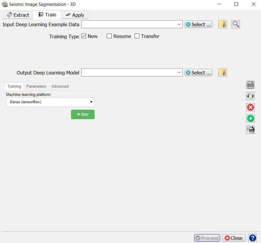
When you already have stored data, you can start in the Training tab with Select training data (Input Deep Learning Example data).

Under the Select training data there are three toggles controlling the Training Type:

• New starts from a randomized initial state.
• Resume starts from a saved (partly trained) network. This is used to continue training if the network has not fully converged yet.
• Transfer starts from a trained network that is offered new training data. Weights attached to Convolutional Layers are not updated in transfer training. Only weights attached to the last layer (typically a Dense layer) are updated.

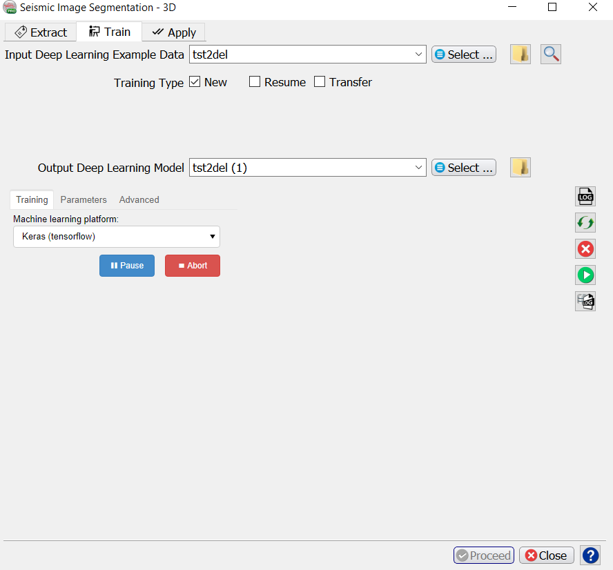
After the training data is selected the UI shows which models are available. For seismic image workflows we use Keras (TensorFlow).

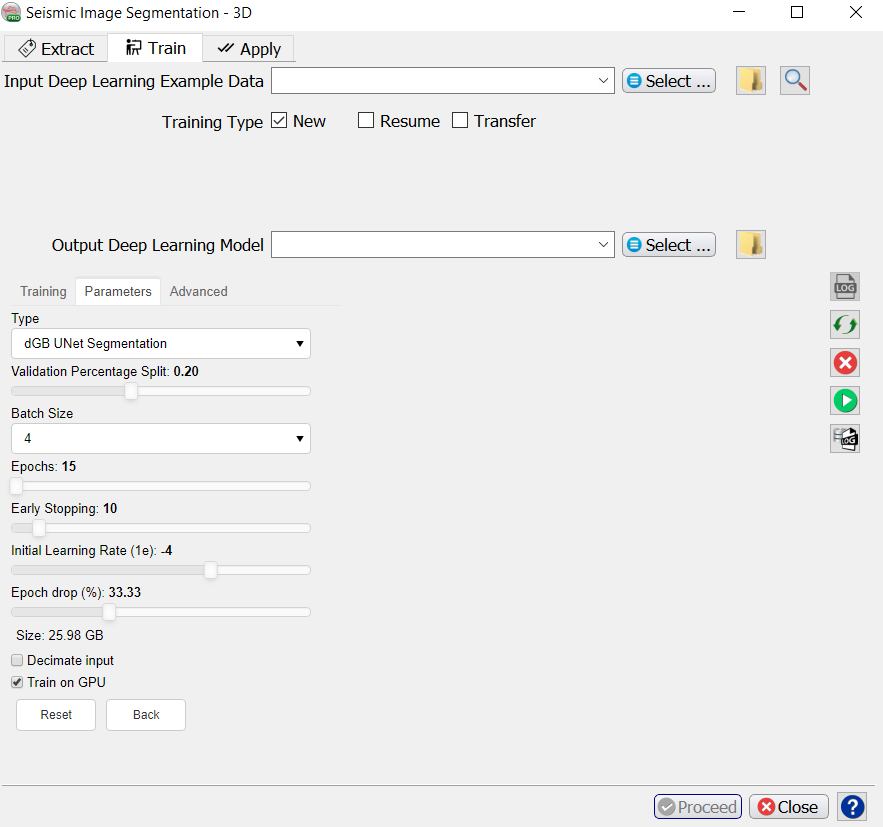
Check the Parameters tab to see which models are supported and which parameters can be changed.

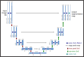
The dGB Unet Segmentation is an auto-encoder - decoder type of Convolutional Neural Network. The architecture is shown schematically below.

The following training parameters can be set in the Parameters tab:

Batch Size: this is the number of examples that are passed through the network after which the model weights are updated. This value should be set as high as possible to increase the representativeness of the samples on which the gradient is computed, but low enough to have all these samples fit within the memory of the training device (much smaller for the GPU than the CPU). If we run out of memory (raises a Python OutOfMemory exception), lower the batch size!

Note that if the model upscales the samples by a factor 1000 for instance on any layer of the model, the memory requirements will be upscaled too. Hence a typical 3D Unet model of size 128-128-128 will consume up to 8GB of (CPU or GPU) RAM.

Epochs: this is the number of update cycles through the entire training set. The number of epochs to use depends on the complexity of the problem. Relatively simple CNN networks may converge in 3 epochs. More complex networks may need 30 epochs, or even hundreds of epochs. Note, that training can be done in steps. Saved networks can be trained further when you toggle Resume.

Early Stopping: this parameter controls early stopping when the model does not change anymore. Increase the value to avoid early stopping.

Initial Learning rate: this parameter controls how fast the weights are updated. Too low means the network may not train; too high means the network may overshoot and not find the global minimum.

Epoch drop: controls how the learning rate decays over time.

Decimate Input: this parameter is useful when we run into memory problems. If we decimate the input the program will divide the training examples in chunks using random selection. The training is then run over chunks per epoch meaning the model will eventually have seen all samples once within one epoch, but only no more than one chunk of samples will be loaded in RAM while the training is performed.

Mixed precision: Mixed precision option has been added to dgbpy for both PyTorch and Keras platform. This allows to train models using a combination of 16-bit and 32-bit precision formats which will optimize GPU memory usage and efficiency. The GPU memory usage can be reduced by 50% and 75% in some cases. It also increases training speed 2 - 3 times on GPUs with Volta or Turing architectures. This doesn't also affect training accuracy or performance.

For more details about what is ‘Mixed precision training’ please refer to:

• Keras documentation: Mixed precision
• NVIDIA documentation: Train with Mixed Precision

After model selection, specify the Output Deep Learning model and press the green Run button. This starts the model training. The Run button is replaced in the UI by Pause and Abort buttons.

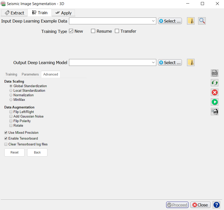
The progress of Keras / TensorFlow runs can be monitored in TensorBoard, which automatically starts up in your default browser. Please note that it may take a few minutes before TensorBoard has gathered the information that is gathered during training. As all TensorBoard information on your machine is retrieved for all current and historic runs it is recommended to clear the TensorBoard log files from time to time. You can do this with the Clear TensorBoard log files toggle before any Run in the Advanced tab.

The progress can be also followed in a text log file. If this log file does not start automatically, please press the log file icon in the toolbar on the right-hand side of the window.

Below the log file icon there is a Reset button to reload the window. Below this there are three additional icons that control the Bokeh server, which controls the communication with the Python side of the Machine Learning plugin. The server should start automatically. In case of problems, it can be controlled manually via the Start and Stop icons. The current status of the Bokeh server can be checked by viewing the Bokeh server log file.

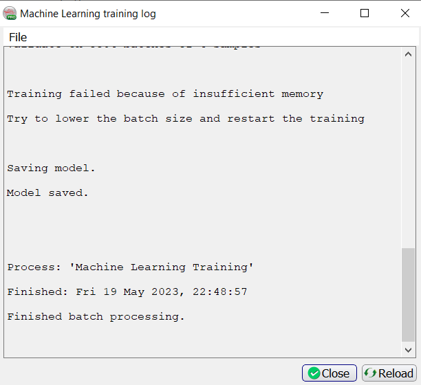
When the processing log file shows “Finished batch processing”, you can move to the Apply tab.

 

Apply

Once the Training is done, the trained model can be applied. Select the trained model and press Proceed.

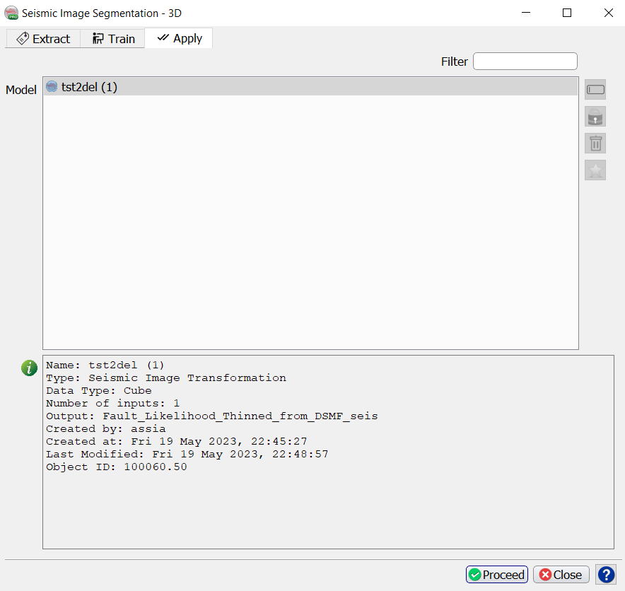
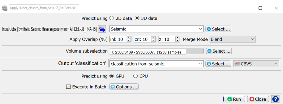
The Apply window pops up. Here you optionally apply to a Volume subselection. You can output a Classification Volume (values 1 to 8 in this case).

Probability is simply the output of the prediction node which ranges between 0 and 1.

Confidence is computed as the value of the winning node minus the value of the second best node.

(You can run on GPU or CPU depending on the Predict using toggle). Running the application on a GPU is many times faster than running it on a CPU. Press Run to create the desired outputs. The image below is taken from a seismic facies Classification cube generated in this way.

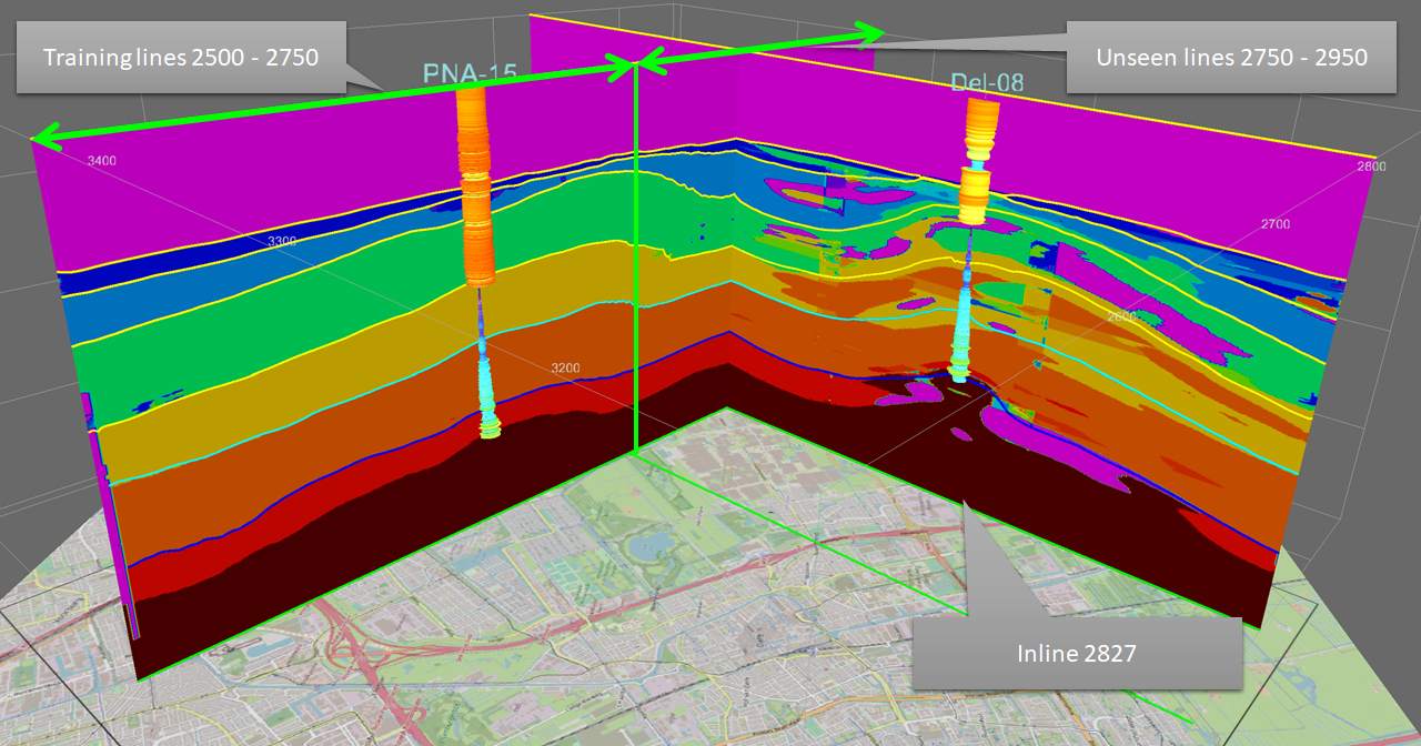
Output of the trained segmentation model: seismic segmentation cube. Input features are extracted from synthetic seismic and Two-Way-Time volumes. Images are 128x128 samples along the inline direction. The model was trained on examples extracted from inlines 2500 - 2750. Prediction is from real seismic and TWT. Model is probably overfitted. Real seismic is more variable than the synthetic data it was trained on. Possible improvements to consider: if possible, create a synthetic model from more real wells, apply data augmentation (i.e. randomly changing input examples, e.g. by cropping, padding, and flipping left-right). Data augmentation requires programming in the Python environment. For more info on programming in OpendTect Machine Learning environment, please visit this webpage.