4.2.2 Create SteeringCube
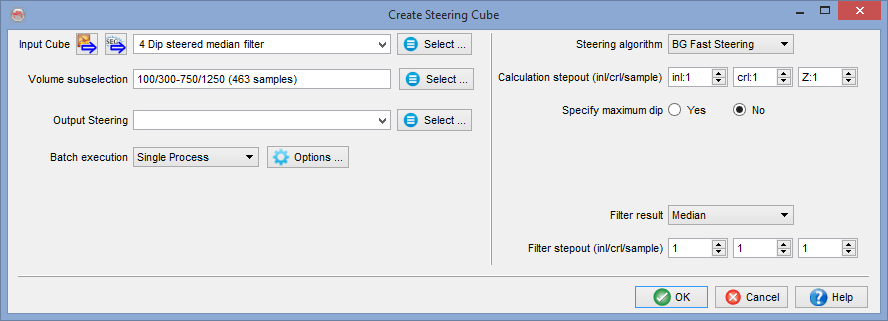
Select the Input Cube (usually a seismic volume) and optionally specify the Volume subselection to process.
Give the SteeringCube to be computed a name under Output Steering.
Under Batch execution specify where the processing is to be done. Single Process means the SteeringCube is processed on the machine you are currently working on. Under Options … you can set the job priority (Linux nice level) from -19 (low) to 19 (top).
Distributed Computing is the recommended mode as computing a SteeringCube is a relatively CPU intensive process. In this mode batch processing is distributed over all computers (workstations and clusters) that are available to the user. The Distributed Computing window is launched after all parameters were set and OK is pressed.
Distributed Computing (processing) is a unique selling point of OpendTect that is not automatically available after a default installation. This mode depends on the network environment and needs to be installed by the system administrator. For details, please see: Chapter 5.5 of the System Administrator’s manual.
OpendTect supports three types of Steering algorithms:
- PCA (new in 6.2)
- Phase-gradient (former BG)
- FFT
PCA (new in 6.2)
Dip Estimation using Principal Component Analysis (PCA)
Reflection dips are estimated using Principal Component Analysis from the seismic amplitude field. This specific PCA uses an Eigen Value Decomposition (EVD) in order to extract the direction (as a 3 component vector) of maximum amplitude changes, as the largest eigen value of the decomposition.
This direction is the normal to the wavefront at any position of the seismic reflector, thus perpendicular to the dip. The second and third eigen values will be located within the plane tangent to the seismic reflection.
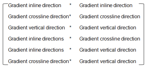
The EVD is applied on a sample by sample basis, using the following six amplitude gradient products, previously computed and smoothed volumetrically using recursive gaussian filters:
The smoothness of the output dip field is entirely determined by the strength of the filters applied to the gradient product attributes prior to the SVD decomposition. Eventually it is not one but three filters that are applied in the vertical, crossline and inline directions consecutively. It is thus possible to adjust each of the three filter strengths independently. Note however that applying a minimum smoothing of 1 in the three directions is essential for a stable estimation of the dip field. Post-processing filtering is usually not required.
Two filtering algorithms are available: the Deriche filter is applied for standard filter sizes (below 32), and the Van Vliet filter for bigger sizes (ϭ = 32 and higher). The runtime, for both filters, is independent of ϭ: Running it with ϭ = 1 takes as much time as with ϭ = 20. For example a processing done with filter size [2, 6, 40] will first apply a Van Vliet filter of ϭ = 40 in the vertical direction. Then a Deriche filter of ϭ = 6 is applied to the previous output in the crossline direction. Finally a Deriche filter of ϭ = 2 is applied in the inline direction to the output.
Because of filters being recursive filters, a larger number of samples in the direction where the filter is applied is required in order to get stable results. As a result the processing engine will automatically load up to 50 additional samples when available in order to stabilize the result. Running the PCA processing in chunks should thus deliver an almost identical result as running the entire dataset at once. However there will be a runtime penalty if the chunk size is set much smaller than 50 inlines per chunk, for instance using Multi-Machine distributed processing.
The EVD may optionally output the relative difference between the first two Eigen Values. When applied on seismic reflections, this attribute is proportional to the "planarity" of the reflection: It will reach a maximum of 1 if the reflection locally coincides with the plane tangent to it, have with be always remain larger or equal to zero.
This optional attribute is stored as a third component of the output SteeringCube. The planarity attribute, similar to a similarity attribute, can be used to weight the inversion-based horizon tracking such as Unconformity Tracker or Multi-horizon HorizonCube.
Phase-gradient (former BG)
Phase-gradient Steering is the recommended algorithm for applying dip-steered filters and to compute dip-steered attributes. Phase-gradient Steering is a quick algorithm developed by the BG-Group. It computes dip in a small sub-volume defined by the step-outs from the gradient of the instantaneous phase. The Phase-gradient algorithm is prone to noise, which can be overcome by adding a median or average filter. The default is to apply a mild median filter with step out 1,1,1.
Optionally, dip computation can be limited to a maximum dip (in us/m).
FFT
FFT Steering computes dip in a small sub-volume defined by the step-outs by searching for the highest energy in the 3D Fourier transformed domain.
Also with FFT Steering, dip computation can optionally be limited to a maximum dip (in us/m) and the results can optionally be smoothed with a median or average filter. The default is not to smooth as smoothing filters can also be applied in a separate step afterwards (see Filter SteeringCubes).
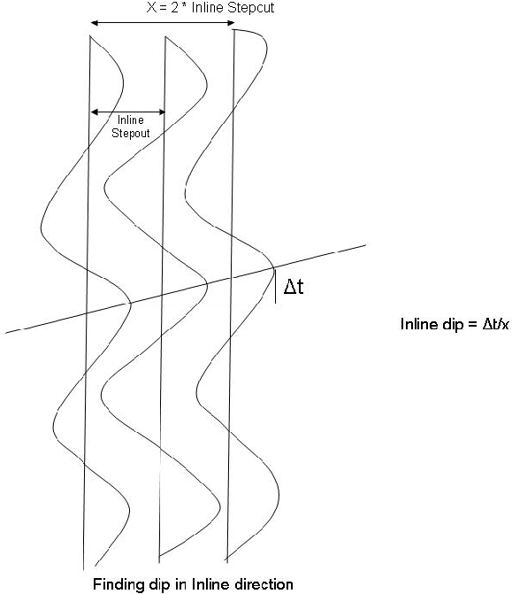
Steering calculates the dip in the inline direction and in the cross-line direction from extrema. All Maxima and Minima are determined on the central trace and two neighboring traces located at the stepout positions. Maxima and minima with the smallest Δt separation (see image) are considered to represent the same seismic event. This results in dip values at all extrema positions. Resampling these values to the seismic sampling rate yields the Steering data at the central trace position.
The maximum dip (us/m) parameter determines the search gate on the neighboring traces within which a maximum, or minimum must be found. The parameter ensures unrealistic dips are found, which may happen in noisy areas.
Also Steering supports optional application of smoothing filters. The default is not to smooth as smoothing filters can also be applied in a separate step afterwards (see Filter SteeringCubes).
The OK button starts the single machine, or multi-machine processing mode. For more information on single and Distributed Computing, open the help menu from the Distributed Computing window.